After concluding my series of essays which hope to bring peace to Palestine, and Israel, I wondered what the walk on the path to peace would look like. Specifically, how would we know how far we’ve come since the cessation of hostilities? After giving it some thought, I came up with a way to subjectively measure the progress. In this essay I shall discuss what it is, starting from a very rudimentary approach, and building on it to make it more sophisticated.
As always, we’ll start with a thought experiment. Take a moment to pause and reflect on what you think the relationship between Moshe, Moosa, and their nations would look like if the hostilities ended. Perhaps you envisioned a utopian outcome where all is blissful, or maybe a more pragmatic outcome which requires both the nations to put in time, and effort to normalise the relationship. In the course of this essay, we shall start with the simplistic, utopian outcome, and then build on it to discuss a more sophisticated, pragmatic outcome.
In its simplest form, an end to hostilities results in peace. In other words, there is war, and then there is peace. In this binary view of the world, an end to the war results in immediate peace. I posit that this is a very naive way to look at the outcome, and I shall explain this using the framework of collective consciousness. In my fifth, and final, essay I mentioned that emotions are both a cause and consequence of events that become a part of the individual, and collective consciousness. Looking at the history of the two nations, it will take some time, and effort for the consciousnesses of both the nations to be at peace with each other. With this in mind, we’ll refine the binary view to include one more outcome - stalemate.
Let us now introduce a state of stalemate that exists between the states of war, and peace. This is a state of equilibruim, a purgatory of sort, which provides the two nations’ consciousnesses sufficient time to heal. We can summarize this by saying that peace is better than stalemate, and stalemate is better than war. In a state of stalemate there is neither war, nor peace but there is the potential for either of the two. This interim period can be used to either prepare for war, or to chalk out a path for ensuing peace. This view of progress, although realistic, is also very mechanical. A state of stalemate is the one of perfect lull where there is neither peace, nor war. An immediate transition to such a state, although possible, seems less plausible given that emotions are a part of collective consciousness. We will refine the view one final time and view the states of war, stalemate, and peace as a spectrum.
Let us now view war, stalemate, and peace as a spectrum. On the far ends are war, and peace, and in the middle is stalemate. Nations of the world who have been at war, and desire to be at peace will have to first, gradually, work towards a state of stalemate. From there, they will have to work, gradually again, towards peace. This, in my opinion, is the most pragmatic way to view the progress after a cessation of hostilities, and fits perfectly well within the framework of collective consciousnesses. The time, and effort it will take to transition to from war to stalemate, and finally to peace, provide the necessary ingredients for the consciousnesses of the two nations to be at peace with each other.
With this view in mind, let us hope that can work towards peace in the land of the prophets.
Thank you for reading.
Footnotes and References
[1] We can view this essay mathematically, too. The first model is a set of ordinal values such that . The second model introduces one more value in the set, , such that . Finally, the third model can be viewed as a range, with values between and , inclusive, where a value of represents stalemate. [2] We can also come up with interactions among nations which can act as milestones to measure progress as they move from war, to stalemate, and then to peace. For example, some amount of trade and commerce can indicate a state of transitioning to a stalemate, whereas completely opening up to trade and commerce indicates transitioning to peace. [3] Combine the two footnotes, and we can empirically measure the state of relations between two nations. Perhaps someday I will write about it and call it ‘Peace, Precisely’.
This is the final essay in my series of essays that aim to bring peace to Palestine and Israel. Like in my previous few essays, I wanted to title it differently but to maintain continuity I shall call it “5th essay”; I had considered “From Moshe to Moosa” or “From Moosa to Moshe”[1] after the inscription on Rambam’s tomb which reads “From Moses to Moses arose none like Moses”[2], a testament to wisdom and intelligence. In this essay I shall try and make an appeal to both emotion and reason, simultaneously, and show why peace is better for both Moshe and Moosa. As is the spirit of this series of essays, I shall handle the subject with sensitivity. If I inadvertently say something insensitive, I apologise from the beginning.
Throughout my essays I have used the lens of collective consciousness to posit that the way forward is peace. In my original essay on collective consciousness, titled ‘Collective Consciousness’, I explain how one is a part of the consciousness of humanity, and how the consciousness of humanity is made up of the consciousnesses of everyone. I also explain how events shape the individual, and collective consciousness. What remained implicit was that emotions, as both the result and cause of events, too, shape consciousnesses.
Let us begin by critiquing my previous essays and calling them hyperrational. I use the word ‘hyperrational’ very consciously because what I have written may be perceived as my asking people on either side to forget whatever is in their consciousnesses, as individuals, and as people of a nation, given my arguments, to work towards peace because that is objectively the better option. To add to the criticism, I wrote in the opening lines of the first essay that I am observing the crisis unfold from a distance and, therefore, carry the credibility of an armchair critic; I am far from hearing a rocket or a bomb explode, or losing a member of my family to this crisis. Although I have tried to defend my position in the second essay, the “if this, then that” approach may seem to be a pure appeal to reason. The classical elements of persuasion suggest that an appeal be made either using the credibility of the speaker, to the emotions of the audience, or to their ability to reason. Much to my dismay, I have the credibility of an armchair critic appealing to the two nations’ ability to reason in an emotionally charged crisis.
In my defense I posit that, using the teachings of Rambam and Ibn ‘Abbas, I shall establish my credibility, and that an appeal can be made to both emotion and reason simultaneously, within the framework of collective consciousness.
Let’s start with a thought experiment. Take a moment to pause and ask yourself what you’d like to be remembered for. Perhaps you’d like to be remembered for your values, for your vocation, for your contributions to a cause you consider worthy, or one of the myriad other things. Your emotions, stemming from your conception of the answer, would lead you in pursuit of bringing it to reality. In other words, your desire to be become an indelible part of humanity’s consciousness would lead you in pursuit of events that bring it to bear. A generalization of this is that the nations of the world would like to be an eternal part of humanity’s consciousness.
We’ll find similar ideas among the medieval Muslim philosophers. They speak of humans as having multiple souls; one vegetal or animal soul, capable only of growth and reproduction without rational thought,[3] and one rational soul.[4] While the former perishes with death, the latter can hope to live on. The true form of the human is, therefore, intellect whereas the body just becomes a conduit for the activation of human potential. The realisation of human potentiality allows one to survive after death, and comes from one’s understanding that these separate souls do not reside in matter. When one contemplates these separate souls, and grasps them, then one is united with them, and becomes eternal. This unification is the closest a human can come to becoming divine, and therefore, is the completion of human perfection, and guarantees immortality, and eternal reward. Ibn Sina, known more popularly as Avicenna, writes about eternal reward, and the felicity of the soul after death in his Kitab al-Najat, The Book of Deliverance, which is a treatise on the soul. He writes that the divine philosphers desire to attain the felicity gained from the unification of the souls than corporeal felicity.[5] He then writes about the difficulties of grasping such a pleasure by giving the example of a eunuch who does not crave the pleasure of intimacy because he has never experienced it, and does not know what it is. This, Ibn Sena writes, is our situation regarding the pleasure whose existence we know but cannot concieve.[6]
Take a moment and pause on the similarity of looking at yourself, and others, from the perspective of many consciousnesses, and that of many souls. I’ll borrow the idea of the felicity of the soul, and propose a felicity of the consciousness that applies to individual, and collective consciousness. I posit that, unlike what Ibn Sena writes, it is indeed possible to experience such bliss. In the context of these essays, however, I shall look at the felicity of the nations of Moshe, and Moosa.
Like in my previous essay, I shall draw upon the sayings of Rambam, beginning with his self-perception. He describes himself to one of his students by saying “You know well how humbly I behave towards everyone, and that I put myself on a par with everyone, no matter how small he may be.” The approach that he had towards his students, and followers was of gentleness, and pragmatism.[7] In my previous essay I had mentioned that Rambam was a polymath who had studied medicine, and astronomy. He considered that the science of astronomy is the hallmark of a civilized nation. In Dalalat al-Ha’irin, The Guide for the Perplexed, in the context of astronomy, he writes that “our nation is a nation that is full of knowledge and is perfect (milla ‘alima kamila), as He, may He be exalted, has made it clear through the intermediary of the Master who made us perfect, saying: ‘Surely, this great nation is a wise and understanding people.’”[8] I’d like to extrapolate from this, with utmost sensitivity, respect, gentleness, and pragmatism, that Rambam considered the Jewish nation as the one of wise and understanding people. The felicity of the nation shall be found, therefore, in his sayings. To contrast this with Ibn Sena’s saying, what Rambam says is both conceivable, and achievable.
We shall now take a look at some of the verses from the Quran, and the sayings of the Prophet (pbuh) to see what would bring felicity to the Muslim consciousness. I am going to focus on those verses, and sayings which find common ground with what has been mentioned above, while also trying to convey the overall picture of the Islamic faith. I shall cherrypick some verses from the Quran, but it is my sincere belief that they shall be within their context. A chapter of the Quran is called “Surah” or “Surat”, and I shall use that to maintain fluency of sentences. The first two verses comes from Surat An-Nisa verse 36 and 37 and state what it means to be a Muslim. They read as follows “Worship Allah ˹alone˺ and associate none with Him. And be kind to parents, relatives, orphans, the poor, near and distant neighbours, close friends, ˹needy˺ travellers, and those ˹bondspeople˺ in your possession. Surely Allah does not like whoever is arrogant, boastful, those who are stingy, promote stinginess among people, and withhold Allah’s bounties. We have prepared for the disbelievers a humiliating punishment.” The verses of the Quran are usually studied in conjunction with the Seerah, the life of the Prophet (pbuh), as his sayings expound on what has been revealed in the verse. One can find many of his sayings about the rights of parents, neighbors, orphans, etc. and on charity, and it is a condition of the Islamic faith, for those who are capable, to donate a percentage of their excess wealth every lunar year, the Zakat. The second verse comes from Surat Ta-Ha, verse 114 and reads “Exalted is Allah, the True King! Do not rush to recite ˹a revelation of˺ the Quran ˹O Prophet˺ before it is ˹properly˺ conveyed to you, and pray, “My Lord! Increase me in knowledge.”” While both a minor admonition, and an advise to the Prophet (pbuh), one can glean the wisdom in asking Allah for increasing one’s knowledge. Finally, I’ll quote hadith 224 from Ibn Majah, a saying of Prophet (pbuh), which says that “Seeking knowledge is an obligation on every Muslim.” The felicity of the nation shall be found, therefore, in what has been revealed to, and said by the Prophet (pbuh). To contrast this with Ibn Sena’s saying, what is mentioned in the Quran and the hadith is both conceivable, and achievable.
Having mentioned the two verses, and the hadith, it is clear that there is a thread that ties the consciousness of the two faiths and that is the one of humility, gratitude, and pursuit of knowledge.
I shall now return to the original premise of the essay and that was to establish my credibility, and to simultaneously make an appeal to reason and emotion. To address the first, I shall merely repeat the sayings of Rambam and Ibn ‘Abbas and that is to take the truth, and by extension wisdom, wherever it comes from. I make no claims to be wise, but I do make a claim to have spoken the truth. Having quoted Rambam, the Quran, and the Prophet (pbuh), I have made an appeal to the emotions of the two nations. Having borrowed from Ibn Sena, I have tried to state that felicity of consciousness, a state of emotion, is achieveable. It, therefore, stands to reason that we make an attempt to attain that which was stated. In the light of the unfolding crisis in the world of Moshe and Moosa, the only path forward to bring this to reality is peace. As I have stated in my previous essays, it is a difficult walk, but what lies at the end makes it worth it.[10]
I’ll end my essays by quoting the last part of Khutbat-ul-Haajah, Sermon of Necessities, that Prophet Mohammed (pbuh) would use as the opening to his sermons. These are two verses from the Quran, one after the other, that exhort the believers to speak the truth, and to remember to follow Allah and his Prophet (pbuh). The verses of Surat Ahzab verse 70-71 are as follows.
“O believers! Be mindful of Allah, and say what is right. He will bless your deeds for you, and forgive your sins. And whoever obeys Allah and His Messenger, has truly achieved a great triumph.”
I hope and pray that as a believing Muslim I have spoken that which is right, and kept my duties to Allah and his Prophet (pbuh).
Amma B’ad. After that.
Footnotes and References
[1] Page 153, Stroumsa S. Maimonides in his world: Portrait of a Mediterranean Thinker. Princeton University Press; 2011. [2] Wikipedia contributors. Maimonides - Wikipedia [Internet]. 2024. Available from: https://en.wikipedia.org/wiki/Maimonides [3] APA Dictionary of Psychology [Internet]. Available from: https://dictionary.apa.org/vegetative-soul [4] Page 153, Stroumsa S. Maimonides in his world: Portrait of a Mediterranean Thinker. Princeton University Press; 2011. [5] Page 154, Stroumsa S. Maimonides in his world: Portrait of a Mediterranean Thinker. Princeton University Press; 2011. [6] Page 155, Stroumsa S. Maimonides in his world: Portrait of a Mediterranean Thinker. Princeton University Press; 2011. [7] Page 113, Stroumsa S. Maimonides in his world: Portrait of a Mediterranean Thinker. Princeton University Press; 2011. [8] Page 113, Stroumsa S. Maimonides in his world: Portrait of a Mediterranean Thinker. Princeton University Press; 2011. [9] The translation of the Quran is from The Clear Quran by Dr. Mustafa Khattab. The text was copied from quran.com. [10] Perhaps if this essay were any shorter I would have written about the story of Yusuf (Joseph), the son of Yaqub (Jacob, Israel), as it exemplifies patience, grace, forgiveness, and provides an additional thread that the two nations together. It is the 12th chapter of the Quran, and I highly recommend you, the reader, to read the translation as you listen to the original recitation. https://quran.com/12. Writing about it would have allowed me to provide one more example through which I could make an appeal to emotion, and reason, simultaneously, to show that path forward is in peace.
In this essay we shall look at the life of Prophet Mohammed (pbuh). I wanted to title the essay as either “Pathway to Peace from the life of the Prophet” or “Patience and Perseverence from the life of the Prophet”. However, it shall be titled “4th essay” to maintain continuity. While there are entire books, both classical and contemporary, that are written about his life, we shall look at it thematically. There are no citations in this essay because my singular source is Ar-Raheeq Al-Makhtum, The Sealed Nectar, which is a contemporary book on the seerah, the life of the Prophet (pbuh). I have taken every care to be as sensitive as I can, but if I inadvertently say anything insentitive, I apologise from the beginning.
Let’s begin with a thought experiement. I would like you to consider your perception of the Prophet (pbuh), whatever it may be. I hope that by the end of the essay, I will have demonstrated that he is, in fact, a prophet of mercy, and that his life demonstrates, realistically, a path to peace despite the challenges encountered along the way. I shall begin with two verses from the Quran, and then begin to go through the life of the Prophet (pbuh) by dividing it into distinct phases. My hope is that such an overview, for the purpose of this series of essays, shall suffice. I do, however, recommend you to read The Sealed Nectar, should you want to read the seerah in relatively more detail.
The first verse is verse 107 from Surat Al-Anbya, and is the premise of my essay. It reads “We have sent you ˹O Prophet˺ only as a mercy for the whole world.” This is in contrast to the popular perception of the Prophet (pbuh) as a warlord. Although he did go to war, they were far from his purpose in life, as we shall see. The second verse is verse 21 of Al-Ahzab and reads “Indeed, in the Messenger of Allah you have an excellent example for whoever has hope in Allah and the Last Day, and remembers Allah often.” As we shall see, when we look at ‘Ām al-Ḥuzn, the Year of Sorrow, it was the Prophet (pbuh)’s hope in Allah that allowed him to persevere through the difficult times, as is also evident from his prayer in Ta’if.
We shall begin by looking at Arabia at the time of the Prophet (pbuh) as it is important to understand the religious, cultural, political, and genealogical backdrop in which he preached the message of Islam.
We begin by looking at the lineage of the Prophet (pbuh). As the story of Abraham has it, he had two sons, Ismail (Ishmael), and Ishaq (Issac). Ismail, and his mother Hajer (Hagar), were left in Arabia by Abraham after Sarah got jealous that Hajer gave birth to a child. Arabs at the time were divided into tribes, and the tribe of the Prophet (pbuh), the Quraish, traces its lineage back to Ismail.[1]
Most Arabs followed the religion of Abraham which is to worship one God, and associate none with him. However, with time they turned to paganism and idolatory. This began when one of the cheifs brought back an idol, named Hubal, from Syria when he saw the Amalek worshipping it, and placed it in the middle of the Ka’bah, the house of Allah in Makkah. Soon, there were more idols placed in and around the Ka’bah. Slowly paganism spread in all of Arabia, and became the predominant religion.
The political situation in Arabia was the one of tribal rule where each tribe had a leader, chosen from among them, who enjoyed complete respect and obedience, similar to a king. The tribes, however, were disunited and were governed by tribal rivalry, and conflicts; there was a lack of a unified government.
Arabian society had a variety of socioeconomic levels and showed a world of contrasts. The status of women, for example, is the one where this becomes most apparent. Women in the nobility were held in high regard, and enjoyed a significant degree of free will. They could be so highly cherished that blood would easily be shed in defense of their honour. Then there were women of another social strata where prostitution, and indecency was rampant; the details have been left out for the sake of decency. While some Arabs held their children dear, others buried their female children alive due to their fear of poverty, and shame. There was, however, a strata of men and women who lived a life of moderation. Another aspect of the Arab life was that of a deep-seated attachment to one’s tribe; unity by blood was a principle that bound the Arabs into a social unit. Avarice for leadership, despite descending from one common ancestor, led to tribal warfare and led to fragile inter-tribal relationships. Their impulse to quench their thirst for blood was restrained by their devotion to some religious superstitions, and some customs held in veneration. The custom of abstaining from hostilities in the four sacred months provided a period of peace, and allowed them to earn their livelihood.
There were also admirable traits of the Arab society. For example, hospitality towards guests was of utmost importance and there was nobility attached to it. They were hospitable to a fault, and would sacrifice their own sustenance for a cold, or hungry guest. Similarly, keeping a covenant was taken seriously so much so that one would not avenge the death of his children just to keep a covenant. The proceeds of gambling, surprisingly, were donated to charity.
Take a moment to pause and reflect on the Arab society in pre-Islamic Arabia. This period is referred to as the period of jāhilīyah, meaning ignorance. This is the society in which the Prophet (pbuh) was born, raised, lived, and preached, and it is easy to imagine why a message of monotheism, devotion, chastity, and generosity would be met with resistance, and even war.
We shall now look at the life of the Prophet (pbuh) in four phases: the pre-Islamic life in Mecca, the post-Islamic life in Mecca, life in Medina, and the conquest of Mecca. These divisions are my own, and have been chosen as they, for the purpose of this essay, convey the complete picture of his life.
Prophet Mohammed (pbuh) was born in Mecca, in the Banu Hashim sub-tribe of the Quraish, to Aminah, and Abdallah. As was the custom, he was sent away to be raised by bedouin wet nurses, away from the city, so that he may learn to speak purer Arabic, and grow up healthier. The bedouins were known for their fleucncy of language, and for being free from the vices that develop in sedentary societies. Before being sent away, Prophet Mohammed (pbuh) lost his father. He stayed with the wet nurses till he turned four or five. When he turned six, his mother passed away, and his care was entrusted to his grandfather Abdul-Muttalib, who was more passionate towards him than his own children. Abdul-Muttalib passed away when the Prophet (pbuh) was eight, and his care was entrusted to his uncle Abu Talib.
In his early youth, the Prophet (pbuh) worked as a shepherd. At age 25 he went as a merchant on behalf of Khadija, his future wife, to conduct business for her, in exchange for a share of the profits. She had heard of his honesty, and offered him a higher share than she did to the previous men she had employed. Upon his return, she noticed an increase in her profits, and heard of his honesty, sincerity, and faith from her aide who had accompanied him. She expressed her desire to get married to the Prophet (pbuh) to her friend, who conveyed the news to him. He agreed, and they were subsequently married. It is from her that he has all his children save one. It was during this period of his life that he earned reputation of being Al-Ameen, the trustworthy.
Take a moment to pause and reflect on the pre-Islamic life of the Prophet (pbuh). Here is a description of his early years in The Sealed Nectar that I will quote verbatim, which I believe aptly summarizes his early years. “He proved himself to be the ideal of manhood, and to possess a spotless character. He was the most obliging to his compatriots, the most honest in his talk and the mildest in temper. He was the most gentle-hearted, chaste, hospitable and always impressed people by his piety-inspiring countenance. He was the most truthful and the best to keep covenant.” Finally, I’ll quote Khadijda who said “He unites uterine relations, he helps the poor and the needy, he entertains the guests, and endures hardships in the path of truthfulness.”
We shall now move on to the part of his life in Mecca after the start of prophethood. This part of his life lasted close to 13 years.
Of the habit of the Prophet (pbuh) was contemplating in solitude. He would take with him some Sawiq (barley porridge), and water, and head to the cave of Hira’. He would spend his time, and especially Ramadan, to worship and contemplate on the universe around him. His heart was restless about the moral evils, and the abandonment of the faith of Abraham that were prevelant among his people. It was the preliminary stage of his prophethood. At the age of forty that he received the first revelation, when Jibreel (Gabriel) appeared to him in the cave. The first revelation had left him so horrified that he ran back to his house, and asked Khadija to cover him. He then narrated the incident to her. She proceeded to take him to her cousin who had accepted Christianity, and the Prophet (pbuh) recalled the incident to him, too. It was here that he was informed that his encounter was divine, and that the angel that appeared to him was the one that appeared to Moses. He was also told of the hardships that lie ahead, and how he would be cast out by his own people. Khadija’s cousin passed away a few days after this conversation. Ibn Hisham, the writer of the earliest, and most authoritative text on the seerah, reports that during the incident of the revelation, Jibreel informed the Prophet (pbuh) of his prophethood.
The first few years were spent preacing privately, and the verses of the Quran focused on sanctifying the soul, and telling Muslims to forego the glamor of life. They also gave a vivid account of heaven and hell. Prayer, Salah, was mandated two times a day. Among the early converts to Islam were those close to the Prophet (pbuh), and the slaves. While the pagans of Quraish paid no heed to the spread of the message during its early years, the later years were filled with animosity. There are detailed accounts of torture, and persecution of Muslims. To portray the gruesomeness of what the early Muslims had to endure, I shall speak of one such incident and that is of Sumaiyyah, the mother of Ammar Ibn Yasir. She was impaled with a spear, driven through her privates, for refusing to leave Islam. There were attempts made to assassinate the Prophet (pbuh) himself, and at one point in time his whole tribe was boycotted for continuing to offer him protection. The Prophet (pbuh) instructed some of the converts to migrate to the Christian kingdom of Abyssinia because he knew that the king was just, and would do right by his subjects.
This phase of his life was also marked by the toughest year, called ‘Ām al-Ḥuzn, the Year of Sorrow, which was the tenth year of prophethood. In this year he lost his uncle, Abu Talib, his wife Khadija, and was stoned after he invited the leaders of Ta’if to Islam, in hopes of finding a haven away from Makkah. He then made a supplication which I shall mention next to show his hope and faith in Allah, as indicated in the earlier part of the essay.
“O Allâh! To You alone I make complaint of my helplessness, the paucity of my resources and my insignificance before mankind. You are the most Merciful of the mercifuls. You are the Lord of the helpless and the weak, O Lord of mine! Into whose hands would You abandon me: into the hands of an unsympathetic distant relative who would sullenly frown at me, or to the enemy who has been given control over my affairs? But if Your wrath does not fall on me, there is nothing for me to worry about. I seek protection in the light of Your Countenance, which illuminates the heavens and dispels darkness, and which controls all affairs in this world as well as in the Hereafter. May it never be that I should incur Your wrath, or that You should be wrathful to me. And there is no power nor resource, but Yours alone.”
The silver lining of the Year of Sorrow was his finding support among people of Yathrib, the city that would later be called Medina.
Take a moment to pause and reflect on the Makkan phase of the life of the Prophet (pbuh). It is the one of persecution, expulsion, and of a search for a place to call home. As we will see in the Madani phase, this will become the backdrop in which he establishes the city of Medina, goes to war, returns to Makkah as a conquerer, and completes the religion of Islam to bring back that which Abraham had taught his children.
The Madani part of his life lasted 10 years. After having made Hijrah, emigration, to Medina, Prophet (pbuh) started establishing it as a city-state; his sight was always on Makkah. Those that made the journey with him are called the Muhajiroon, the Immigrants, and the ones who gave them refuge are called the Ansar, the Helpers. The Quraish had done everything they can to prevent people from undertaking the journey to Medina since such a departure would sully their honor. The Ansar knew that by accepting the Prophet (pbuh) in their midst they would have a possibility of war, and that did come to pass. As time unfolded, the Muslims went to war against the Makkans multiple times, and with each war the size of the Makkan army kept getting larger, and in one of the battles the Muslims found their martyrs mutilated. Eventually, they reach the treaty of al-Hudaybiya, which would seize the hostilites on both sides.
However, this is also the time when the Prophet (pbuh) makes the the Night Journey, the Isra’ and Mi’raj, where he travels to Jerusalem, and then ascends to the heavens. During this journey he is greeted by prophets of old including Isa (Jesus), Abraham, and Moosa (Moses). The hadiths, and the verses in the Quran, regarding the Night Journey describe in vivid detail what he saw. The Prophet (pbuh) mentions Sidrat al-Muntaha, the lote tree under the throne of Allah to which everything ascends. He also mentions two heavenly rivers, and two worldly rivers; the worldly rivers are Nile and Euphrates. It is in his ascension that he meets Allah, in a way that He deems fit, and is given the ordainment of fifty prayers for his followers. Upon his return from meeting Allah, Moosa asks him to go back, and ask for the them to be reduced. Eventually, after asking Allah a few times, the Prophet (pbuh) accepts the five daily prayers as the Divine decree.
Take a moment to pause and reflect on this phase of his life. I am going to talk about one last incident, and that is the conquest of Makkah, that took place after the Quraish breached the treaty of al-Hudaybiya.
After making complete preparations for the conquest, the Prophet (pbuh) departed with an army of 10,000. The news-blackout that the Prophet (pbuh) had imposed gave the Quraish no opportunity to prepare against the oncoming army. However, to not take them by surprise, the Prophet (pbuh) asked the Muslims to light cooking fires on all sides, so that the Quraish had an opportunity to prepare. Abu Sufyan, the leader of the Quraish, who was yet to accept Islam, sought an audience with the Prophet (pbuh). The Prophet (pbuh) then granted the people of Mecca general amnesty, and to honor Abu Sufyan said “He who takes refuge in Abu Sufyan’s house is safe; whosoever confines himself to his house, the inmates thereof shall be in safety, and he who enters the Sacred Mosque is safe.”. Upon entering Makkah as a conquerer, the Prophet (pbuh), proceeded to the Ka’bah, and destroyed the idols. He later addressed the people of Quraish and recited the verse of the Quran which reads “O humanity! Indeed, We created you from a male and a female, and made you into peoples and tribes so that you may ˹get to˺ know one another. Surely the most noble of you in the sight of Allah is the most righteous among you. Allah is truly All-Knowing, All-Aware.” He then asked what they thought is the treatment that they shall be meted with, and they said that they expect nothing but goodness from him. To this he said “I speak to you in the same words as Yusuf (Joseph) spoke unto his brothers: He said: ‘There is no blame on you today’, go your way, for you are freed ones.”
Take a moment to reflect on the aftermath of the conquest of Makkah in which the Prophet (pbuh) forgave everyone. The ones he forgave are the ones who mocked him, persecuted him, stoned him, and went as far as mutilating the body of his uncle. In his life we find a practical approach to finding lasting peace and serenity. The path ahead for both Moshe, and Moosa is to emulate the Prophet (pbuh), and say that there is no blame on the other.
This is me looking for peace in the land of the prophets, by citing the life of the prophet of mercy.
Footnotes and References
[1] I am going to, consciously, gloss over the Qahtani and Adnani distinction for the sake of simplicity. The footnote exists as an acknowledgement to the nuance. Suffice to say, Ismail is an Adnani Arab who married into the Qahtani Arabs. Such details are better suited for an intermediate or advanced seerah class.
In the last two essays I mentioned the examples of Rambam, and Prophet Mohammed (pbuh), and how they pave the way for long-term peace. In this essay I’d like to introduce you to Rambam, and hopefully convey my admiration and reverence for him. While I originally wanted to title this essay as either “Revering Rambam” or “An Ode to Rambam”, I decided to call it “3rd essay” to make it a continuation of the previous two. In the same spirit, I shall handle this subject with sensitivity, and respect. If I inadvertently say something insensitive or disrespectful, I apologise from the beginning. The intention of this essay is to introduce you, the reader, to who I consider to be the most influential Judaeo-Arabic minds.
Let’s begin this essay with a thought experiment. I’d like you to close your eyes and imagine yourself standing in a park, or a cafe, or a meadow, or some place you consider beautiful. I’d like you to appreciate the beauty in its entirety, and then focus on the individual elements like the sights, the sounds, the smells, etc. that together make the scene beautiful. I posit that the beauty of Rambam’s thinking, like that of yours, is in the coalescence of individual elements. These are elements from his Jewish heritage, and those from his exposure to Islamic, and to some extent Christian, cultures.
Let us now look at Rambam’s life and works. I’ll start by attempting to piece together his life from whatever information I have. By the end of this essay, I hope to have conveyed what I suggested in the previous two, which is that Moshe and Moosa share a common thread of humanity through Rambam.
Moosa Ibn Maimoon al-Andalusi, also known as Moshe Ben Maimon ha-Sefaradi in Hebrew, known as Rambam, was born in the Arabic metropolis of Córdoba in 1135 or 1138. Descending from a long line of rabbanic scholars who preserved their genealogy, along with their titles, going back seven generations, he was one of two sons. He was quite fond of his younger brother, David, whom he educated and, as we will see later, trusted in affairs of business.[1]
Rambam was born towards the end of the golden age of Jewish culture in Spain, when the power of the governing dynasty of the Almovarids began to dwindle. They had granted Jews and Christians the dhimmi status. When we return to the Constitution of Medina, which Prophet Mohammed (pbuh) dictated, it states that any Muslim, even the weakest, is permitted to provide protection (dhimmah) to another person, and that it is binding on the rest of the Muslim Ummah. While the Constitution intends for it to be binding on Muslims living in Medina at the time, we can extrapolate that if the ruler of a nation grants dhimmi status to a group of people then it becomes binding on his subjects.
The Almohads rose to power, signaling the end of the golden age. Chroniclers describe the challenges of life as a Jew during the Almohad conquest, as well as persecution, when Abd al-Mu’min, the Almohad ruler, launched his conquest of North Africa and Andalusia.[2] Rambam’s family was forced to leave Cordoba, and eventualy moved to Fez, and then to Fustat.[3] During this period, Rambam was studying medicine, astronomy, rabbinic literature, and serving as an apprentice rabbinic judge.[4]
Rambam engaged in the precious stone trade in Fustat until the death of his brother David, who died in the Indian Ocean while doing business.[5] The Maimonides family had entrusted David with their savings in the hopes of growing their wealth. Rambam was deeply affected by his brother’s death, and in a letter found in the Cairo Geniza, a collection of Jewish manuscripts discovered in a storehouse (gheniza) of a synagogue in Fustat, Rambam laments how a tremendous sorrow had befallen him.[6]
The death of David led to financial hardship for the family of Rambam who had to take up the profession of the court-physician. Fustat, by now, was under the Ayyubid dynasty.[7] He confirms that he had studied both the theory and practice of medicine, and perhaps may have been preparing himself to become a physician. He did eventually gain renown for his profession, and even remarked that his attendance as a physician on Salah ad Deen’s courtesans was a fortunate turn in his life.[8] He even attendeed Salah ad Deen himself[9] and continued as a court-physician after his death.
He continued as a physician and passed away in 1204 in Fustat. His final resting place is in the city of Tiberias in Israel, and is one of the most important sites of pilgrimage.[10]
Take a moment to pause and reflect on the life of Rambam as that of, first and foremost, someone following the Jewish faith, and an intellectual living in the Mediterranean world. For a historian, however, the term “Mediterranean world” is problematic because the cultural boundaries are flexible; they can go from Italy in the West to Palestine in the East.[11] However, we can say that the Mediterranean world of the Islamic middle ages was one of economic relationships, exchange of books, science, and ideas, all of which contributed to the multifaceted universe in which Rambam lived.[12] We’ll take a quick look at only two of his sayings to demonstrate the brilliance of his ideas, beginning with another thought experiment; offering an overview of his work is beyond the scope of this essay.
The first saying, the thought experiment, serves as a guide for how we can think about Moshe and Moosa. In his book Dalalat al-Ha’irin, The Guide for the Perplexed, he states that when the process of thought is interrupted, “at first thought” (bi-awwal fikra), it is prone to create ideas that are incorrect, incomplete, or even dangerous.[13] Pause for a moment and reflect on your thoughts regarding Moshe and Moosa. I believe that, as Rambam stated, your first thought (fikra) was to see the other, depending on whose side you are on, in the most negative light. In the spirit of what has been mentioned in the Guide, we can take a minute to pause, reflect, and let the initial thought fade away to make place for the next.
Finally, I’d like to quote him from Commentary on the Mishnah. In that he writes that one should listen to the truth regardless of who says it; Isma’ al-haqq mi-man qalahu.[14] This is similar in structure to the advise of Ibn ‘Abbas, the cousin of Prophet Mohammed (pbuh) who said that one should take wisdom wherever it comes from, even if it comes from the non-wise. It is possible Rambam may have read this in Kindi’s Al Qutayba[15] since Jewish philosophers at his time read the work of their Muslim contemporaries. What matters less is whether he read it in the book, or if the idea was commonplace. What matters truly is the principle of reaching for knowledge and truth, whatever the source may be; this is the thread that ties Rambam with ‘Ibn Abbas.
This is me as I continue to look for peace in the land of the prophets.
Footnotes and References
[1] Page 4, Davidson HA. Moses Maimonides: The Man and His Works. Oxford University Press, USA; 2010. [2] Page 11, Davidson HA. Moses Maimonides: The Man and His Works. Oxford University Press, USA; 2010. [3] Page 8, Stroumsa S. Maimonides in his world: Portrait of a Mediterranean Thinker. Princeton University Press; 2011. [4] Page 20, Davidson HA. Moses Maimonides: The Man and His Works. Oxford University Press, USA; 2010. [5] Page 9, Stroumsa S. Maimonides in his world: Portrait of a Mediterranean Thinker. Princeton University Press; 2011. [6] Wikipedia contributors. Maimonides - Wikipedia [Internet]. 2024. Available from: https://en.wikipedia.org/wiki/Maimonides [7] Page 9, Stroumsa S. Maimonides in his world: Portrait of a Mediterranean Thinker. Princeton University Press; 2011. [8] Page 35, Davidson HA. Moses Maimonides: The Man and His Works. Oxford University Press, USA; 2010. [9] Page 36, Davidson HA. Moses Maimonides: The Man and His Works. Oxford University Press, USA; 2010. [10] Wikipedia contributors. Tomb of Maimonides [Internet]. Wikipedia. 2024. Available from: https://en.wikipedia.org/wiki/Tomb_of_Maimonides [11] Page 9, Stroumsa S. Maimonides in his world: Portrait of a Mediterranean Thinker. Princeton University Press; 2011. [12] Page 5, Stroumsa S. Maimonides in his world: Portrait of a Mediterranean Thinker. Princeton University Press; 2011. [13] Preface, Stroumsa S. Maimonides in his world: Portrait of a Mediterranean Thinker. Princeton University Press; 2011. [14] Page 11, Stroumsa S. Maimonides in his world: Portrait of a Mediterranean Thinker. Princeton University Press; 2011. [15] Page 12, Stroumsa S. Maimonides in his world: Portrait of a Mediterranean Thinker. Princeton University Press; 2011.
I’d shared the first essay with my close friends in hopes of receiving feedback. I heard back from one of them saying that perhaps my essay, although hopeful, came a few years too late, and that it would be difficult to explain my stance to the people on either side, given everything that has transpired in the last few decades. This second essay is in defense of the first, and I shall try to explain why peace is still the way forward. As always, I shall handle this topic with utmost sensitivity, and I apologise if I inadvertently say things that come across as insensitive.
Let’s recap the first essay. We saw Moshe and Moosa, two 15 year old kids on either side of the conflict, who grow up to find themselves facing each other to defend what they consider to be their home. We then looked at the examples of Rambam, and Prophet Mohammed (pbuh) to see what the path to peace would look like. The story of Moshe, and Moosa remained incomplete. Like in the first essay, we will wind the clock forward a decade and look at the various ways in which things can unfold. Finally, we will posit that peace is still the only option.
Take a moment to reflect on your position on this issue. I hope that in the course of this essay I am able to allay any doubts you may have, and convince you to act towards making peace.
The first point that my friend had raised was that my essay is a few years too late. I’d like to address this by using the weiji (危机) metaphor that views a crisis as both a perilous situation, and a catalyst for change. It is the severity of the crisis that prompted me to write the essay, which will hopefully become the catalyst for lasting peace.
The second point that my friend had raised was that both the nations have tried to make peace in the past, and are yet to reach it. I’d like to respond by saying that the negotiations and treaties that were signed leave a lot to be desired. There is still lingering resentment and animosity on either side that shows from time to time. Also, the consequence of breaking down of the peace process is eternal war. Therefore, it stands to reason that attempts be made to ensure that it does not come to pass. It may, from the consciousnesses of the two nations, and of humanity, feel like rolling a boulder up the hill only to find it roll back down. To this I say that this is the only good pursuit there is.
The final point that my friend had raised was that perhaps Moshe would not want peace. This requires a more nuanced answer and we need to look beyond the consciousnesses of the two nations, and into the ones of those that surround them. We will look at these consciousnesses, and wind the clock forward a decade and reflect on the consequences of Moshe’s decisions. I’d like to retierate that I firmly believe in there being a common thread of humanity that ties Moshe and Moosa together, as we saw in the first essay, and that both Moshe and Moosa want peace and security for their homeland.
Let us now look at the theater of war.
Moshe’s nation, Israel, shares its border with 4 other nations. It has, at different points in time, been at war with its neighbors. All of them, however, share the consciousness of faith with Moosa. Further to the East is the nation where Moosa’s religion of Islam originated, and further to the West is another nation observant of the same faith. While Moshe’s nation, by itself, is militarily strong, and has powerful allies, there is a risk of conflict opening on multiple fronts.
In contrast, Moosa lives in Gaza, a small strip of land which is surrounded by Moshe’s nation on 2 sides, the sea on 1 side, and a neutral nation on 1 side which observes the same faith as he does.
Take a moment and reflect on the intricacies of the situation. In isolation, the war between Moshe and Moosa can be framed as a geopolitical dispute over borders. A borader look at the war reveals, given Moshe’s neighbors, that it can turn into a geo-religious-political dispute.
We’ll now look at two possible outcomes and wind the clock forward a decade to see how they may unfold. One, Moshe wins and manages to subdue Moosa, and his people militarily. Two, Moshe and Moosa end up in a stalemate. I posit that both of these outcomes are lose-lose for Moshe, and Moosa, and we shall see why.
Let us look at the first scenario where Moshe wins using military means, and manages to subdue Moosa and his nation. Such a victory is very myopic, and as counterintuitive as it may sound, goes against the original objective of securing his homeland. Given the collective consciousness of faith that Moosa’s nation shares with Moshe’s neighbors, near and far, there is now an ever-present threat of going to war with them, and perhaps simultaneously. It may happen either immediately, in the near future, in the far future, or never at all; the threat, however, shall remain. If it does happen, it risks drawing other nations of the world into it.
Also, military victory would come at a cost of significant civilian casualties to Moosa’s nation. While Moshe and his nation wins, they will forever be remembered, in the collective consciousness of humanity, as those who inflicted pain on those who had nothing to do with the war.
Those that do live through the war may now be left with no place to call home; Moshe did to Moosa’s people that which was done to his, and perhaps it will weigh heavily on him.
Take a moment and reflect on this outcome.
Let us now look at the second scenario where Moshe and Moosa end up in a stalemate.
In this scenario, neither Moshe nor Moosa win. After a long, drawn out war, Moshe and Moosa reach an agreement of sort that ends hostilities temporarily. In the course of the war, Moosa loses his wife and 2 daughters. I posit that such a scenario makes the next war even worse than the previous.
With time the military technology would advance, and with that the weapons of Moshe and Moosa. The nations that share the consciousness of faith with Moosa would do everything they can to help him, both militarily and diplomatically. Similarly, Moshe’s allies would help him militarily and diplomatically. Moshe would not have, still, achieved the objective of securing his homeland. Similar to the situation discussed previously, it has infact deteriorated the security of his nation. There is now a looming threat of Moosa retaliating with more fervor, and of drawing other nations into it.
Take a moment and reflect on this outcome.
I hope that this essay addresses any doubts as to why peace is the only way forward. The examples of Rambam, and Prophet Mohammed (pbuh) were deliberate as they tie Moshe and Moosa together. Let us envision a future where Moshe and Moosa sit across a table, say Salam Alaikum or Shalom Aleichem to the other, as children of Abraham and of humanity, heal the wounds that have been inflicted, bridge the divides that have been created, and bring their people a step closer to eternal peace. The road ahead is long, and paved with thorns, but what lies at the end is worth the walk.
This is me still looking for peace in the land of the prophets. Thank you for reading.
I recently read in a book that the Chinese word for crisis is weiji (危机). It consists of two characters: wei (危) meaning danger, and jei (机) meaning a point of inflection. In other words, a crisis is both a perilous circumstance and a catalyst for change. If handled correctly, a crisis can become an essential component and a powerful force for good. In this essay I am going to look at the Palestine and Israel crisis as weiji. I will draw on the collective consciousness of people on both sides to provide a stance that, I believe, will pave the way for long-term peace. This essay is my perspective, and I am only one of many people seeing the crisis unfold from a distance. I understand that this is a sensitive subject, and I will take every care to handle it as such. I am sure that I will inadvertently say things that people on both the sides will find insensitive, and for that I apologise from the beginning.
I’ll begin by introducing Moshe and Moosa, two young boys on either side of the conflict, and wind the clock forward a couple of times, one decade at a time, to show how they develop their consciousnesses. However, I’d like you to start by reflecting on your own position on the Palestine and Israel crisis, and hopefully watch it transform as we progress through the essay.
Let me introduce Moshe. He is 15 years old, and lives in the beautiful city of Tel Aviv. Like many kids his age living in the modern state of Israel, Tel Aviv is the only home he has known. He dreams of growing up and going to the university to follow in the footsteps of Jonas Salk. He is aware of the ever-present state of tension, and has heard the sirens go off as rockets land in his home city. In his history class he has studied about the Holocaust, the migration of the Jewish people in search of a home, and how that led to the formation of the modern state of Israel. He has also heard about the destruction of the Temple of Solomon from his rabbi. His consciousness as a young 15 year old kid is that of hopes and dreams, and his consciousness as an Israeli Jew is that of persecution, expulsion, and the search for a place to call home.
Let me now introduce Moosa. He, too, is 15 years old and lives in the beseiged city of Gaza. Like many kids his age living in under siege, Gaza is the only home he has known. He dreams of growing up and going to the university to become a surgeon after having seen the effects of shrapnel. He, too, is aware of the ever-present state of tension, and vividly remembers fighter jets and exploding bombs. He studies in a dilapidated school, and in his history class he has studied the formation of the modern state of Israel. He has heard the stories of the Naqbah from his grandfather, who wears the key to their old house around his neck. He yearns to go back and see the house his grandfather grew up in. His consciousness, as a young 15 year old kid, is that of hopes and dreams, and his consciousness as a Palestinian Muslim / Christian is that of persecution, expulsion, and of yearning to go back to the land his family once called home, and perhaps to play among the olive trees.
Take a moment to pause and reflect on the original position you started with. We shall now wind the clock forward a decade to a time where both Moshe and Moosa are 25 years old.
Moshe studied [1] medicine at the prestigious Tel Aviv University. He runs a successful practice, and is married to the love of his life that he met at the university. In the last 10 years, however, his country has come under attack twice. He now worries that, in the future, his children may not have a place to call home. He plans to run for political office with the hope of influencing policies and ensuring the security of Israel. His consciousness is that of someone looking out for his people; this is afterall his homeland.
Moosa got married to the girl who lives two houses from where he lives; they went to school together. He, too, is a doctor and runs a medical practice. In the last 10 years his city has twice witnessed a blockade, once for 90 days at a stretch. During this period there was only a trickle of food, and medical supplies; he had to scrounge for syringes, bandages, and medicines. He is among the many people who have lived through the blockade, including many young children. He has seen kids develop symptoms of post traumatic stress, and worries that the same will befall his children in the future. He plans to join the local political movement in hopes of bringing international pressure on the state of Israel. His consciousness is that of someone looking out for his people; this is afterall the only place left to call home.
Take a moment to pause and reflect on the original position you started with. We shall now wind the clock forward a decade to a time where both Moshe and Moosa are 35 years old.
Both Moshe and Moosa ran for political office, and now hold the highest position there is. While Moshe turns West to look for allies, Moosa turns East. They both use diplomatic, and military means to secure the place they call home. Their consciousnesses are of their nations, etched indelibly with the events of the last two decades. Nations of the world watch as the days unfold, and take the side of either Moshe or Moosa. People on each side portray the other in the most negative light.
Take a moment to pause and reflect on the original position you started with.
We begin to see the inflection point when we look at the crisis from the perspective of collective consciousnesses; there is a common thread of humanity that connects both Moshe and Moosa. To make this clear, I’d like to introduce one more Moshe or Moosa, someone I admire, and that is Moosa ibn Maimoon (Moshe, the son of Maimoon), also known as Rambam (רמב״ם) or more commonly as Maimonides. He was a prominent philosopher and polymath among both the Jewish and Islamic worlds.
Maimonides was born in either 1138 or 1135 in Andalusia[2]. During his early years, he studied Torah with his father and became interested in science and philosophy. He read Greek philosophers’ writings that were available in Arabic, as well as Islamic sciences and traditions. In 1148, however, after the Almohads conquered Cordoba, Maimonides’ family chose exile. He moved to Fez in Morocco, and eventually to Fustat in Egypt. He took up the profession of physician, for which he gained renown, and later became the physician of Salah ad Deen (Saladin). Among his notable achievements are treatises on medical and scientific studies, and the systematic codification of the Halakha, the way of life for the Jewish people.
Rambam’s life exemplifies a consciousness that offers peace to both Moshe and Moosa.
Take a moment to pause and reflect on the original position you started with.
While what is inscribed in Moshe and Moosa’s consciousnesses, as well as those of their nations and humanity, will endure, it is up to them to determine what will be etched in the future. I will now posit that the route to reconciliation stems from the life of Prophet Mohammed (pbuh), and provides a thread of humanity that can bind the consciousnesses of the two nations. His life, like that of Moshe, Moosa, and Rambam was the one of persecution, expulsion, and of finding a place to call home. He eventually found it in the city of Medina.
After migrating to Medina, Prophet Mohammed (pbuh) dictated what is called The Constitution of Medina.[3]. It mentions the rights and duties of the different tribes, Muslim and Jewish, and envisions a multi-religious Medina. While the complete text of the Constitution is left out for the sake of brevity, we shall look at two statements that truly capture the essence of this essay.
“They (Muslims) shall constitute a separate Ummah as distinguished from the people (of the world) … And the Jews of Banu ‘Awf shall be considered as one Ummah along with the believers — for the Jews their religion, and for the Muslims theirs, be one client or patron.”
The word the Constitution uses is Ummah which translates to a community. However, a closer look at the word reveals its profundity. Ummah dervies from Umm or Amm which means mother. Ummah is, therefore, people who are so close that they might have descended from the same mother. This is an apt description for the followers of the two Abrahamic faiths; one descends from Ishaq (Issac), and the other from Ismail (Ishmael). It is within the realm of reason to view the people of both the faiths coexisting side-by-side in harmony.
We can now reframe the Palestine and Israel conflict as the one where two Ummahs lay claim to the land of their common ancestor Abraham. This, in my opinion, is the most peaceful way to look at the crisis.
Let us now critique the essay by saying that the juxtaposition between Moshe and Moosa is wrong, and that the examples of Rambam and Prophet Mohammed (pbuh) are out of place. Perhaps this criticism is correct, and all we have is an amalgamation of random thoughts that have been weaved together. In it’s defense, we can say that the alternative is eternal tension, animosity, and war.
The path ahead, should the passage of time unfold itself to bring this essay into reality, is long and arduous. Whatever wrong, perceived or genuine, that has been to both the sides can only be partially undone. However, there is also hope of lasting peace and serenity in the intertwined consciousnesses of both Moshe and Moosa. The walls that they have built will take time to come down but it only takes a kind word, an extended hand, and a gracious smile to connect the two hearts.
This is me looking for peace in the land of the prophets. Thank you for reading.
Footnotes:
[1] I have but the faintest idea at what age people graduate medical school. [2] I am using Wikipedia as my source. Maimonides. [3] I am using Wikipedia again. The Constitution of Medina.
Let’s begin with some reflection. I’d like you to recall the last time you were in a public place, such as a café, a restaurant, or a crowded train station. What did you observe? Pause for a moment and consider it. In this essay, we’ll look at a perspective on the world that I believe will help you understand the intricacy of the interconnected world in which we live.
Imagine yourself as a dot on a piece of paper; this is who you are in the big picture. Your views, life experiences, and perceptions all shape who you are. They come together to build your consciousness. Let us now place a few additional dots around you to represent your family. Individuals in your family have separate consciousnesses, but because they share experiences, they now have a shared consciousness. Birthdays, graduations, births and deaths, and so on are all regular life events that everyone in the family will remember. This is the collective conscience of a family, or more broadly, a group of people. We shall continue to generalize until we have a collective consciousness of humanity.
Let us now draw a box around your family, followed by a few nearby boxes with dots. This represents the neighborhood. People in the neighborhood have similar experiences, which are determined by a variety of characteristics such as socioeconomic status, ethnicity, shared or conflicting values, and so on. Each neighborhood possesses its own consciousness. A village, town, or city is formed when many of these neighborhoods are combined together. When several such villages, towns, and cities are combined, they form a province, and when numerous provinces are combined, we have the modern nation with well-defined borders.
The nation’s collective consciousness is molded by past and present events, as well as its vision for the future. These events might be positive, such as major achievements, or negative, such as wars, famines, epidemics, acts of terror, and so on. The consciousness of many such nations together constitutes humanity’s collective consciousness, which extends back throughout time.
The framework we’ve looked at offers a highly humanistic perspective on individuals and humankind as a whole. We’ve looked at a pretty static picture of collective consciousness in which individuals are represented as dots, but in the next sections, we’ll look at a more dynamic view in which the dots move around to interact with other dots. Like in previous sections, we’ll begin with one dot, the individual, and work our way up to a collection of dots, the nation.
Assume that each dot is now colored according to its national flag and moves freely, interacting with other dots. The very first dots to come into contact are those within the family. As a dot moves further away, it may come in contact with dots from its own neighborhood, from another province, or from a different nation altogether. When a dot interacts with another dot, an exchange of ideas occurs. As a result, there will be dots with similar ideas and those with differing ideas; one will come across others who have similar beliefs. These ideas can be political, religious, economic, moral, or any other topic on which one has an opinion. In other words, dots with similar consciousness prefer to attract each other. Finally, a nation is a collection of many consciousnesses that function as one. However, spontaneous interaction among groups of dots with no organization produces friction and chaos. As a result, guiding principles must exist to determine how consciousnesses interact. These compose the nation’s constitution. We can now begin to conceive of a nation’s laws as principles influencing migrating consciousness, and are themselves created from the collective consciousness the nation. The interaction among nations, either for war or for trade, can be viewed as interactions among consciousnesses of that nation and just as laws govern interaction among individuals, they govern interaction among nations.
As a result, you, the reader, have your individual consciousness as well as a connection to the wider human consciousness. Your deeds and the life you build will be indelibly inscribed in the memory of time.
In critique of my own train of thought, I’d want to point out that the framework I provided is overly simplistic and fails to account for the endless variety of existence. For example, it does not discuss the life of an orphaned child. However, in its defense, the model may be expanded to explain it as well.
Thank you for reading my pseudo-philosophical post. I’d like to reiterate the question: what do you see when you stand in a crowded area?
My fiancee recently asked me why random things happen in life. For example, someone winning a lottery. The best answer I could come up with was that it is divine preordainment; we’re both religious. However, I’ve been thinking about a more mathematical approach to view life, and its randomness. In a nutshell, I view life as a set of random variables. This post is banter, so please take it as such.
Let’s view life as a set of discrete, and continuous random variables; . These infinite variables could represent multiple things. For example, median income, level of education, IQ, EQ, Haleema, etc. Any given person’s life is a collection of a subset of values of these variables. We could represent my life as . Let us now define a random process which can alter the set of values within ; values can be added, removed, or updated. As an example, the value of median income can be changed by .
We can now introduce a continuous variable (goal) which takes on values between and , inclusive. This is a measure of how close one is to achieving what they want in life. This can either be affected by a single random variable from , or it can be a composite score derived from multiple variables. Someone may view their life as the outcome of a single variable, or as a composite score derived from multiple variables. Everyone has a baseline value of that makes them feel fulfilled and happy; the more carefree may be okay with a lower value, where as the more careful may want a higher value. This is similar to risk tolerance when making financial decisions. There is the target value of which one would like to achieve; this means they’ve achieved their goal in life.
We’ll introduce one final variable (ability), and that is, as you may have guessed, a measure of person’s abilities. This takes on values between and , inclusive. It is a measure of a person’s ability to alter the value of given any random subset of variables. For example, a person with high value of may be able to maintain the baseline value of , or be able to move it towards the target value regardless of the values of the subset of .
This is the lens with which I view the world, and I hope you had a good time reading this post.
A common requirement for a data warehouse is to store data from third-party sources like SaaS tools. For example, results of surveys conducted by Product or Marketing teams, or status of JIRA tickets. While most of these tools provide an option to export data, it could be very limited. For example, they’d only allow downloading it as a CSV file from their dashboard as a one-off download. Some of them provide APIs to export data which is a lot more convenient. Of those that do provide a direct integration with a warehouse, it’d be with the commercial ones like Snowflake. If we’re using a different warehouse, it is going to take some engineering effort to periodically get this data.
In this post we’ll look at how we can streamline this ingestion. As always, we’ll use open-source technologies to do this. Like in my previous post, we’ll use Doris as our data warehouse. We’ll use the open-source tool Meltano to fetch data from a Github repository. While this is not going to fully replace the need to write custom code, it will help us benefit from the collection of open-source connectors that come with Meltano.
Setting things up
Like in my previous post, my setup consists of Docker containers for running Doris locally. There’s a Postgres container that runs as a part of this setup. We’ll install Meltano, and ingest data into a Postgres database. We’ll then create a catalog in Doris that points to the data ingested in Postgres. While it may be possible to ingest the data directly into Doris by letting Meltano write it to S3, I find it much easier to write it to a database.
Getting started
For the purpose of this post we’ll will be modifying the example on Meltano’s website to ingest data from Github to Postgres. Meltano is available as a pip package and I already have a Conda environment in which it is installed. I’ll gloss over the steps that show how to create a Meltano project for the sake of keeping the post brief, and jump right into the ones where we add the Github extractor, the Postgres loader, and configure them.
Let’s start by adding the loader, and the extractor plugins.
We’ll then configure them one-by-one, starting with the Github plugin. We’ll add the repository we’d like to fetch data from, and the auth token that will be used to authenticate with Github.
1
2
meltano config tap-github set repositories '["thescalaguy/blog"]' meltano config tap-github set auth_token '...'
Next we’ll configure the Postgres plugin. We’ll ingest the data into a schema called “github” in the “ingest” database.
1 2 3 4 5 6
meltano config target-postgres set user postgres meltano config target-postgres set password my-secret-pw meltano config target-postgres set database ingest meltano config target-postgres set port 6432 meltano config target-postgres set host 127.0.0.1 meltano config target-postgres set default_target_schema github
Finally, we run the pipeline.
1
meltano run tap-github target-postgres
A successful run of the pipeline will create a whole bunch of tables in Postgres. One such table is “repositories”, and we’ll query it next.
1
SELECT id, repo, org, name FROM repositories;
The query above gives us the following row.
1 2 3
| id | repo | org | name | |----------|------|-------------|------| | 95359149 | blog | thescalaguy | blog |
We’ll now create a catalog in Doris that points to the database in Postgres. To do this we need to execute the CREATE CATALOG command. Notice that we’ve specified the driver_url that points to Maven. This is a lot easier than manually downloading the JAR, and making it available in the Docker container.
We have one last step before we can query the data, and that is to fix a few symlinks in the containers. It looks like the code is looking for CA certificates at a location different than where they actually are. From what I could glean from the documentation, perhaps the base image has changed and the paths need to be upadted. In any case, here’s how to fix it both in the FE and BE containers by docker exec-ing into them.
Now we’ll run a SELECT query. Notice how we’re writing the FROM clause; it is catalog.schema.table.
1 2
SELECT id, repo, org, name FROM meltano.github.repositories;
There are, however, limitations to what we can read from the Postgres table. Some of the column types are not supported. Changing the query to SELECT * will raise an error that “topics” column is not supported. We can describe the table in the catalog to check which of the columns cannot be read.
1
DESC meltano.github.repositories;
The result shows “UNSUPPORTED_TYPE” next to “topics” column. This is perhaps because Doris uses MySQL protocol and there’s no equivalent mapping bewteen Postgres and MySQL for that type. One way to mitigate this is to create a new column using Meltano’s stream_maps, and parse it in Doris.
That’s it. That’s how we can ingest data from third-party systems into Doris.
I have a few requirements when choosing a SQL IDE. I’d like to use something that is relatively modern, has good support for a wide variety of databases, and allows making charts and graphs. I looked at Metabase, TablePlus, DBeaver, DataGrip, and Apache Superset. All of these tools have a feature or two that is missing in the other. For example, DataGrip allows creating entity relationship diagrams that make it easy to understand how the tables are related to each other; many of the tools do not have this feature. The free version of TablePlus allows creating only one set of charts; Metabase and Superset allow creating many of these. For my day-to-day requirements, as you may have guessed from the title of this post, Apache Superset is the best fit. This post shows how to quickly set up Superset using Docker Compose.
Why Superset
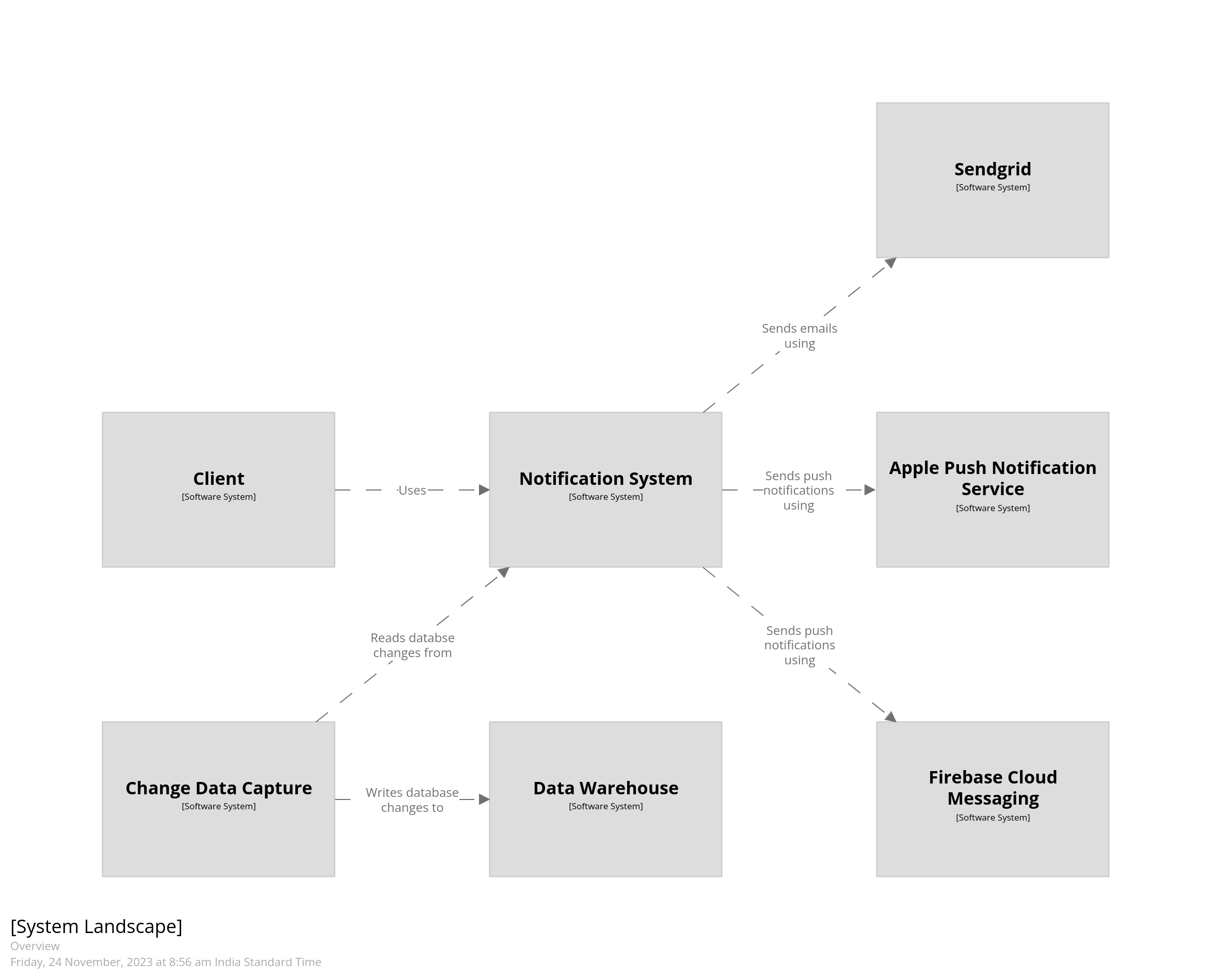
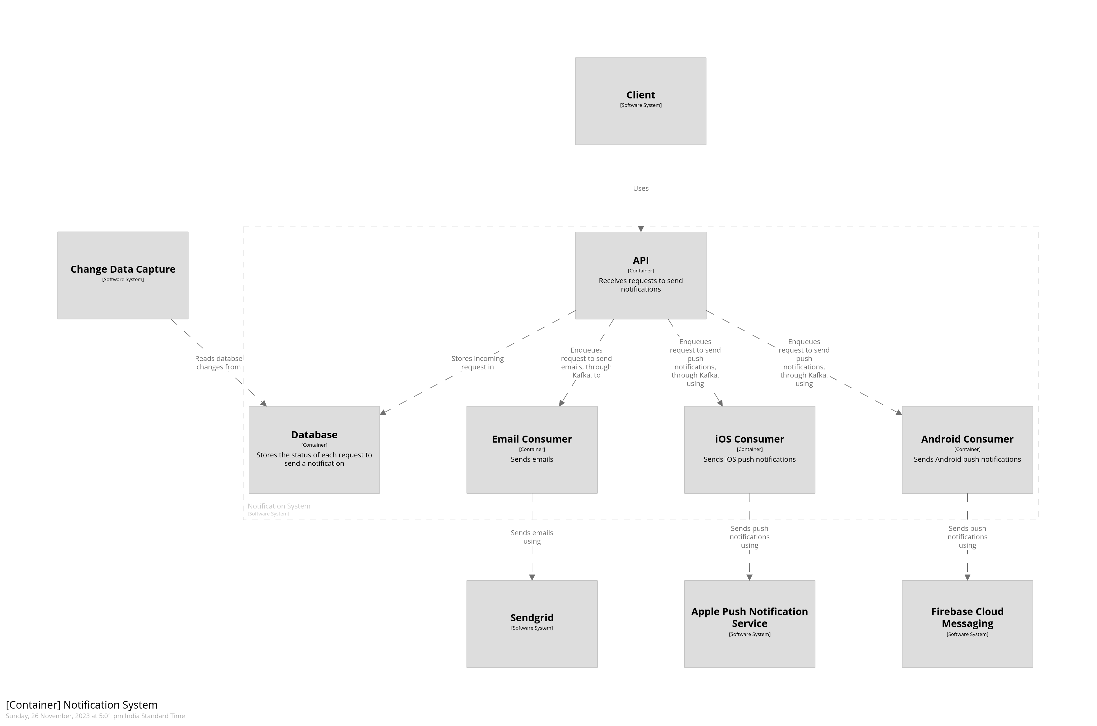
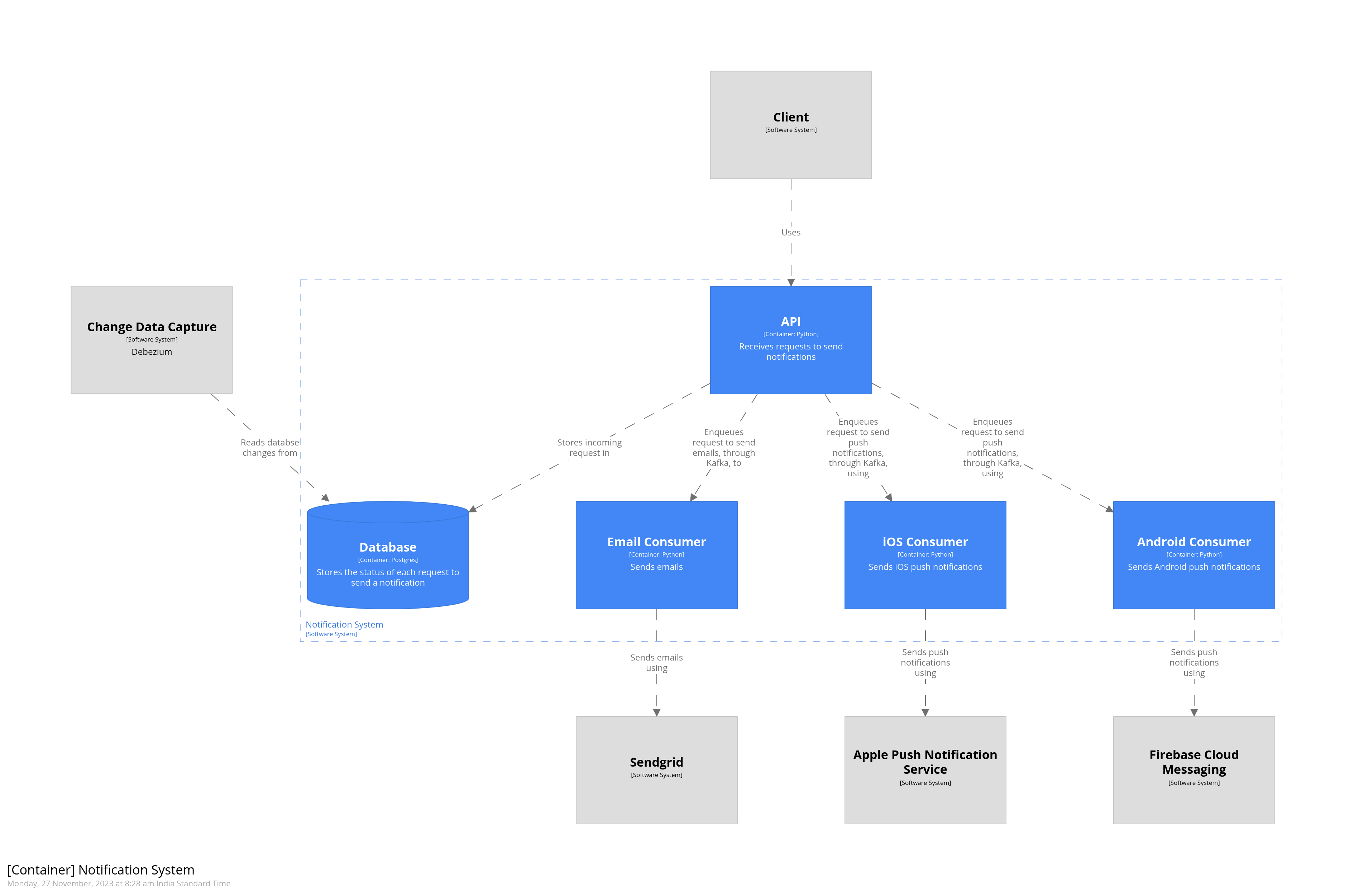
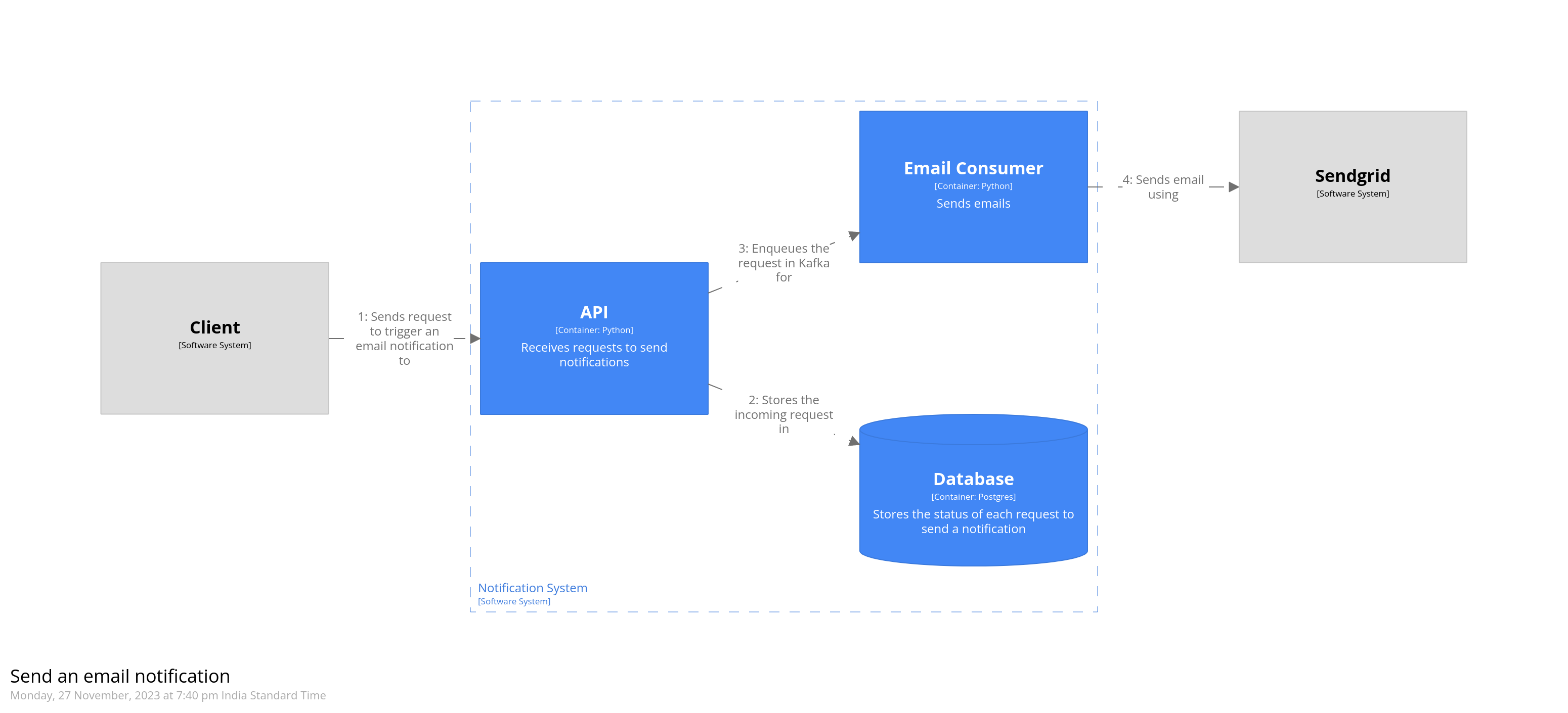
One of the things I often need to do is to monitor the performance of a system. For example, building upon the previous post where I talked about a hypothetical notification delivery system, counting how many notifications are being sent out per day, both as an aggregate metric across channels, and per-channel. This can be tracked by generating StatsD metrics, and charting them in Grafana. However, chances are that we’d need to display them to the customer, and also to other non-technical stakeholders. To do this we’d need our systems to generate records in the database, and have these be stored in a data warehouse that we can eventually query. This is where Superset is useful; it has built-in IDE that allows exploratory data analysis, and the ability to create charts once we’ve finalised the SQL query. The query can then be made part of the application serving analytics, or the BI tool that is used to by the stakeholders.
Another reason is that it is an open-source, actively-developed project. This means bug fixes and improvements will be shipped at a decent cadence; we have a tool that will stay modern as long as we keep updating the local setup.
Finally, because it is an open-source project, it has good documentation, and a helpful community. Both of these make using a technology a pleasant experience.
Setting up Superset
Superset supports a wide vartiety of databases. However, we need to install drivers within the Docker containers to support additional databases. For the sake of this example, we’ll install the Snowflake driver. To set up Superset locally we need to clone the git repo. Let’s start by doing that.
1
git clone https://github.com/apache/superset.git
Next we navigate to the repo and add the Snowflake driver.
1 2 3
cd superset echo"snowflake-sqlalchemy" >> ./docker/requirements-local.txt echo"cryptography==39.0.1" >> ./docker/requirements-local.txt
I had to add the cryptography package manually because the first time I set up Superset, logs showed that database migrations did not run becasuse it was missing.
Next we checkout the latest stable version of the repo. As of writing, it is 3.0.1.
1
git checkout 3.0.1
Now we bring up the containers.
1
TAG=3.0.1 docker-compose -f docker-compose-non-dev.yml up -d
This will start all the containers we need for version 3.0.1 of Superset. Note that if we add newer drivers, we’ll need to rebuild the images. Navigate to the Superset login page and use admin as both the username and password. We can now follow the documentation on how to set up a data source, and use the SQL IDE to write queries.
One of the GoF design patterns is the facade. It lets us create a simple interface that hides the underlying complexity. For example, we can have a facade which lets the client book meetings on various calendars like Google, Outlook, Calendly, etc. The client specifies details about the meeting such as the title, description, etc. along with which calendar to use. The facade then executes appropriate logic to book the meeting, without the client having to deal with the low-level details.
This post talks about how we can create a facade in Python. We’ll first take a look at singledispatch to see how we can call different functions depending on the type of the argument. We’ll then build upon this to create a function which dispatches based on the value instead of the type. We’ll use the example given above to create a function which dispatches to the right function based on what calendar the client would like to use.
Single Dispatch
The official documentation defines single dispatch to be a function where the implementation is chosen based on the type of a single argument. This means we can have one function which handles integers, another which handles strings, and so on. Such functions are created using the singledispatch decorator from the functools package. Here’s a trivial example which prints the type of the argument handled by the function.
@echo.register defecho_int(x: int): print(f"{x} is an int")
@echo.register defecho_str(x: str): print(f"{x} is a str")
if __name__ == "__main__": echo(5) echo("5")
We start by decorating the echo function with singledispatch. This is the function we will pass our arguments to. We then create echo_int, and echo_str which are different implementation that will handle the various types of arguments. These are registered using the echo.register decorator.
When we run the example, we get the following output. As expected, the function to execute is chosen based on the type of the argument. Calling the function with a type which is not handled results in a noop as we’ve set the body of echo to ellipses.
1 2
5 is an int 5 is a str
When looking at the source code of singledispatch, we find that it maintains a dictionary which maps the type of the argument to its corresponding function. In the following sections, we’ll look at how we can dispatch based on the value of the argument.
Example
Let’s say we’re writing a library that lets the users book meetings on a calendar of their choosing. We expose a book_meeting function. The argument to this function is an instance of the Meeting data class which contains information about the meeting, and the calendar on which it should be booked.
Code
Model
We’ll start by adding an enum which represents the calendars that we support.
1
2
3
4
5
6
import enum
classCalendar(str, enum.Enum): GOOGLE = "google" OUTLOOK = "outlook"
Next we’ll add the data class which represents the meeting as a dataclass.
Finally, we’ll start creating the facade by adding functions which will dispatch based on the value of calendar contained within the instance of Meeting.
Dispatch
We’ll create a registry which maps the enum to its corresponding function. The function takes as input a Meeting object and returns a boolean indicating whether the meeting was successfully booked or not.
Next we’ll add the book_meeting function. This is where we dispatch to the appropriate function depending on the meeting object that is received as the argument.
1 2 3 4 5 6 7
defbook_meeting(meeting: Meeting) -> bool: func = registry.get(meeting.calendar) ifnot func: raise Exception(f"No function registered for calendar {meeting.calendar}") return func(meeting)
To be able to register functions which contains the logic for a particular calendar, we’ll create a decorator called register.
1 2 3 4 5 6 7
defregister(calendar: Calendar): def_(func: MeetingT): if registry.get(calendar): raise Exception(f"A function has already been registered for {calendar}") registry[calendar] = func return func return _
register accepts as argument the calendar for which we’re registering a function. It returns another higher-order function which puts the actual function in the registry. Since the actual logic of the execution is in the decorated function, we simply return the original function func.
Finally, we register functions for different calendars.
1 2 3 4 5 6 7 8 9 10
@register(Calendar.GOOGLE) defbook_google(meeting: Meeting) -> bool: print(f"Booked Google meeting") returnTrue
@register(Calendar.OUTLOOK) defbook_outlook(meeting: Meeting) -> bool: print(f"Booked Outlook meeting") returnTrue
We’ll put all of this code in action by trying to book a meeting on Google calendar.
This prints “Booked Google meeting”, like we’d expect. We can now continue to add more functions which contain logic for specific calendars. Our library can evolve without any change to the exposed interface. It’s also possible to organise functions into their own modules, import the register decorator, and decorate them to add them to the registry. This has two main benefits. One, we keep the code well structured. Two, the code for different versions of the same calendar can stay separated; we avoid having to write if checks to see the calendar version since that can be made part of the enum itself, like GOOGLE_V1.
That’s it. That’s how you can create a facade in Python.
Let’s start with an exercise: ask two of your colleagues to create an architecture for a moderately-complex CRUD app. Chances are that they’d look very different from each other. They’d look different because the notations used to depict different parts of the system, like a database, for example, are different. Additionally, everyone has a favorite tool like DrawIO, LucidChart, paper towel, etc. for drawing these diagrams. This approach only works well for rapid prototyping. The drag-and-drop nature of most drawing tools, and paper towel’s susceptibility to getting lost make documenting large software systems a less-than-pleasant experience.
This post describes how to use code to create software architecture diagrams and then commit them to version control. We’ll look at the process and tools for producing consistent diagrams at various abstraction levels, ranging from high-level to low-level. To achieve this, we will create a fictitious notification delivery system. After reading this you should be able to draw diagrams for your own systems at various levels of detail, and be able to explain them to different types of audiences.
In the first part we will talk about why it is necessary to represent the system at various levels of abstraction. In the second part we will talk about notations we can use to draw our system. In the last part we will work through the notification delivery system and create different types of diagrams for it. If you’re looking for an introduction-by-example, feel free to skip to the third part.
Abstraction
Consider a typical software engineering team. You can categorize the people in the team as “engineers” or “not engineers”. Product managers and other stakeholders would make up the “not engineers” portion of the team. They require a broad overview of the system. Within the engineering team, too, people look at the system at different levels of detail. A junior engineer, for example, would focus on the subsystem they are working on while passing by the other subsystems. A more senior engineer, on the other hand, would be expected to be intimately familiar with many systems. This requires presenting the system at different levels of abstraction, depending on the intended audience.
The C4 model allows us to create such views of the system - from the least to the most detailed. The four C’s of the model stand for context, containers, components, and code. A system is made up of many containers (applications, databases, etc), each of which contains multiple components (various API controllers, etc), which are made up of code elements (individual classes, functions, interfaces, etc.). The diagram below, taken from C4 model’s website, shows how they are arranged in a hierarchy.
Given the hierarchy of the four C’s, we can create diagrams at different levels of abstraction. For example, a high-level diagram which only shows different software systems. The highest-level diagram is called the system landscape diagram. This shows how our system fits into the larger scheme of things. The system context diagram narrows the focus by showing our system and the systems that it interacts with. A container diagram adds more detail by showing the responsibilities of different subsystems that together make up our system. Finally, a code diagram shows the most detailed view consisting of class hierarchies, ER diagrams, etc.
Creating such diagrams is helpful because it lets us communicate effectively. For example, we’d use the system landscape or system context diagram when discussing the scope of changes with the product team. A junior engineer, on the other hand, could work their way through the different types of diagrams to get a sense of how the system works.
Writing code to generate these multiple perspectives of the system is a really convenient method, as you’ll see later in the post. All of the views can be generated automatically by the same code. In comparison, you could use a drag-and-drop tool. However, keeping all the diagrams in sync with each other gets tiresome and error-prone.
Notation
Languages like UML are very heavy on notation. For example, the notation to draw a component diagram is very different from a sequence diagram. In contrast, the C4 model is very light on notation. As a starting point, you could represent different diagrams using boxes and arrows, and then augment them with shapes and colors to convey more information. This makes it easy for different people to understand the diagrams without getting bogged down in notation.
As you’ll see in the example that follows, we’ll start with boxes and arrows. For example, the database would be represented as a grey box. We’ll then change it’s shape and color to make it a blue cylinder.
Example
Now let’s look at our notification delivery system. It consists of a REST API which allows callers to send notifications across various channels like email, SMS, or push notifications. Every incoming request is added to a Kafka topic, depending on the channel of delivery, and is eventually picked up by background consumers. The status of each request is updated in the database. A CDC pipeline reads from this database and stores it into a warehouse. The diagram below gives an overview of what the system would look like.
Getting Started
My tool of choice for creating architecture diagrams as code is Structurizr. It provides a DSL which lets us create C4 model of our systems. When you visit its homepage, you’d find an example of how the same code can generate different views of the system at different levels of abstraction. We will use the open-source version of the tool, called Structurizr Lite, which allows a single person to create, edit, and view diagrams; in other words, there is no collaborative editing. The workflow we are aiming for lets individuals submit architecture diagrams as a part of their pull requests. In the next section, we will create a script which will let us run Structurizr Lite as a Docker container. We will then create the diagram that we saw above using the Structurizr DSL.
start.sh
We’ll start by organizing our Git repository. At the top level is the design folder where we will keep all the Structurizr code. The start.sh script, also at the top level, will launch the Docker container and reference the files in the design folder.
1 2 3 4
. ├── app.py ├── design └── start.sh
The content of the start script is the following:
1 2 3 4 5 6 7 8 9 10
#! /bin/bash
if [ -z $1 ]; then echo"You should provide a file name" exit 1 fi
We pass the name of the file as the first argument when we run the script. It is stored in the /usr/local/structurizr directory of the container which we have mapped to the design folder of our Git repository. When we run the script and the file does not exist, Structurizr creates it for us. This is helpful when we are creating a new diagram. If the file exists, Structurizr will read from it and render the diagrams. Let’s start by creating our first file.
1
./start.sh 001-overview
This will create two files under the design folder. The one we’d like to edit ends with dsl extension and will be committed to the repositiory. It is okay to add the json file to gitignore as that will be generated again when the container runs.
views { systemLandscape notificationSystem "Overview" { include * autoLayout lr }
systemContext notificationSystem "Context" { include * autoLayout lr } } }
Let’s unpack what is going on here. At the top-level is the workspace which is a container for the model and views. A model contains the different pieces of our architecture. This includes the software system we are describing, the people and external systems it interacts with, and the relationships between them. views contains the different levels of abstractions at which we’d like to see the system. Here we’ve defined the system landscape view, and the system context view.
In the model we’ve defined various software systems and the relationships between them. The system that we’d like to diagram is the notificationSystem. At this stage we’ve just added a one-line definition of the system, as softwareSystem, which results in it being rendered as a box in the diagram with its name on it.
We’ll continue to refine this diagram by defining other parts which together comprise the notification system. We will do so by adding them as children of the notification system which we’ve defined in the DSL. In other words, we will add one more level of detail to the system.
Relationships between the different parts of the system are defined using an arrow ->. These can be added as children of a softwareSystem or defined outside of them, as we’ve done above.
Adding more detail
We will now zoom in and add the containers which make up the notification system. We will add the background consumers which consume the notifications enqueued in Kafka and send them to the relevant channel. Update the contents of the dsl file to the following:
# -- Relationships between systems user -> api "Uses" api -> email "Enqueues request to send emails, through Kafka, to" email -> sendgrid "Sends emails using"
api -> ios "Enqueues request to send push notifications, through Kafka, using" ios -> apns "Sends push notifications using"
api -> android "Enqueues request to send push notifications, through Kafka, using" android -> fcm "Sends push notifications using"
# -- Relationships between components api -> db "Stores incoming request in" }
views { systemLandscape notificationSystem "Overview" { include * autoLayout lr }
systemContext notificationSystem "Context" { include * autoLayout lr }
container notificationSystem "Container" { include * autoLayout tb } }
}
Notice that we’ve added components which are children of the notification system. We’ve also changed the relationships to point to these components instead of the parent software system. This keeps the system landscape and the system context diagrams the same but allows us to add a new container diagram to the system. This diagram is shown below.
You can add more detail by creating a component diagram. This will let you show individual parts of your software that perform specific tasks. For example, a REST API controller which handles incoming requests to send notifications. Although possible, it is recommended to add a component diagram only if it adds value. Usually it’d be sufficient to only create a container diagram.
Styling our diagram
The diagram we’ve created so far conveys the architecture. However, the only indication of what is internal to the notification system, i.e. within the scope of the system, is a faint dashed line which groups various components together. Let’s go ahead and style our diagram by making components that are a part of the notification system render with a blue background. We’ll start by creating a few directories under design directory.
We’ve created three directories. styles will contain files which store styling information. icons is where we will keep PNG icons. themes is where we will store predefined themes. This is what the directory structure will look like.
Let’s create default.dsl under the styles directory. The contents of the file are given below.
1 2 3 4 5 6 7 8 9 10 11 12
styles { element "internal" { background #4287f5 color #ffffff }
element "database" { shape Cylinder }
}
Here we are creating a couple of custom elements. We are creating an internal element which has a blue background color, and a database element which is a cylinder. We will then use these elements to style our diagram. Let’s update the dsl file to include these elements. I’m only showing the parts that have changed for the sake of brevity.
We begin by including the styling information using the !include directive under views. Styling information is associated with individual systems and components by using tags. You can combine tags to apply multiple styles. Tags can be specified in-line or as a child of a software system or a component. We’ve specified the internal tag in-line for the api container, and as a child of the db container. Notice how we’ve applied both the internal and database tags to the db container, causing it to be rendered as a blue cylinder. With styling, the container diagram now visually communicates what is within and outside the scope of the notification system.
Dynamic diagrams
The diagrams we’ve created so far are static and only show the structure of the system. Dynamic diagrams allow us to show the flow of information between systems as a sequence of steps. They are like UML sequence diagrams but allow a more free-form arrangement of the various parts of the system. The steps are numbered to show the order in which they happen.
As an example, let’s model how an email notification would be triggered. The API receives a request to send an email. It stores this incoming request in the database, and then puts it into a Kafka topic. The consumer then picks up this request, and sends the email using a third-party system.
Dynamic diagrams are created using the dynamic element under views. To model the scenario mentioned above, we’d add the following to our dsl file.
1 2 3 4 5 6 7 8 9 10 11 12 13 14
views { ...
dynamic notificationSystem { title "Send an email notification" user -> api "Sends request to trigger an email notification to" api -> db "Stores the incoming request in" api -> email "Enqueues the request in Kafka for" email -> sendgrid "Sends email using" autoLayout lr }
... }
The steps are written in the order in which they appear. Numbers indicating their sequence are added automatically by Structurizr. The dynamic diagram for the code we just added is given below.
Deployment diagrams
Deployment diagrams allow us to show how the software will actually run. For example, the various components of the software can be deployed as containers running on a Kubernetes cluster. We’ll start by creating a simple deployment diagram which shows the local development environment. All of the services, except the ones that are third-party, will run on the developer’s laptop.
Deployment diagrams are created by adding a model under model using the deploymentEnvironemnt keyword. Once that is defined, we include it in the views. Let’s model the development environment.
1 2 3 4 5 6 7 8 9 10 11 12 13 14 15 16 17 18 19
model { ... development = deploymentEnvironment "Development" { deploymentNode "Laptop" { containerInstance api containerInstance email containerInstance ios containerInstance android containerInstance db }
We’re creating a node called “Laptop” which will host all the components running on the developer’s local machine. To this we add the various containers. We add another node to contain all the third-party services. Relationships between these are automatically inferred from the container diagram created previously. Finally, we add it to views
1 2 3 4 5 6 7 8
views { ... deployment * development { include * autoLayout lr } ... }
This gives us the following diagram.
We can also depict how the software would be deployed to production. Let’s say that our system is deployed to AWS. Our databse is an RDS cluster, and API servers and email consumers are deployed to EC2 instances. We use Route52 for DNS, and Elastic Load Balancer to forward requests to the API servers. Like we did for the development environment above, we’ll create a deployment diagram. This diagram, however, will be styled some more to indicate the various AWS services.
Structurizr allows importing themes. Themes provide predefined tags which you can use to style elements of your diagram. Themes are added to views. Let’s start by adding the AWS theme.
Next we’ll model the production environment. In the model below, we’re nesting deployment nodes. The outermost node represents the AWS environment as a whole. The next node represent the AWS region. Being able to nest deployment nodes allows us to reuse elements of a diagram. For example, if we had multiple database clusters that were all hosted on Amazon RDS, we could nest them all under a single deployment node representing Amazon RDS.
We’ve added Route52 and ELB as infrastructure nodes, and defined relationships between them. They’re styled using tags that we imported from the AWS theme. These are defined in the JSON that’s returned from the theme’s URL.
You don’t need to add relationships between deployment nodes that host your containers. These relationships are implied from the container diagram that was created above.
Finally, we’ll add the production environment to views.
1 2 3 4 5 6 7 8
views {
    ...
    deployment * production {
        include *
        autoLayout lr
    }
    ...
}
This gives us the following diagram. Notice how adding tags has caused AWS icons to be added and styling to be applied, wherever applicable. This is a very small subset of the overall system. Some of the background consumers, CDC, and warehouse have been omitted.
That’s it. That’s how you can create software architecture using code. I’ve created a Github repository for this blog post which contains the complete code for creating the notification system we discussed above.