Bivariate Linear Regression

In the previous post we built the intuition behind linear regression. In this post we’ll dig deeper into the simplest form of linear regression which involves one dependant variable and one explanatory variable. Since we only have two variables involved, it’s called bivariate linear regression.

Ordinary Least Squares

We defined sample regression function as:

$${Y_i} = \hat{\beta}_1 + \hat{\beta}_2X_i + \hat{u}_i \\\\ {Y_i} = \hat{Y}_i + \hat{u}_i$$

The term is called the residual. If we re-write the sample regression function, we get . The residual then represents how far off our estimated value is from the actual value .^[1] A reasonable assumption to make is that we should pick and such that the sum of is the smallest. This would mean that our estimates are close to the actual values.

This assumption, however, does not work. Let’s assume that our values for are -10, 3, -3, 10. Here the sum is zero but we can see that the first and last predictions are far apart from the actual values. To mitigate this, we can add the squares of the residuals. We need to pick and such that the sum of the square of the residuals is the minimum i.e. is the least.

Again, assuming the values of to be -10, 3, -3, 10, the squares are 100, 9, 9, 100. This sums to 218. This shows us that the predicted values are far from the actual values. is called the residual sum of squares (RSS) or the squared error term.

The method of OLS provides us with estimators and such that, for a given sample set, is the least. These estimators are given by the formula:

$$\begin{align} \hat{\beta}_2 &= \frac{\sum{x_iy_i}}{\sum{x_i^2}} \\ \hat{\beta}_1 &= \bar{Y} - \hat{\beta}_2\bar{X} \end{align}$$

where = , . These are the differences of individual values from their corresponding sample mean or . The estimators thus obtained are called least-squares estimators.

Now that we’ve covered significant ground, let’s solve a sum by hand.

Example

Let’s start by drawing a random sample from the original dataset. The sample I’ve drawn looks like this:

income (X)  expenditure (Y)
        80               65
       100               70
       120               84
       140               80
       160              118
       180              130
       200              144
       220              137
       240              191
       260              150

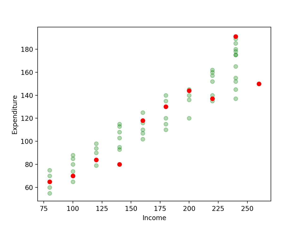
To see how this contrasts with the original dataset, here’s a plot of the original dataset and the random sample. The faint green points represent the original dataset whereas the red ones are the sample we’ve drawn. As always, our task is to use the sample dataset to come up with a regression line that’s as close as possible to the population dataset i.e. use the red dots to come up with a line that’d be similar to the line we’d get if we had all the faint green dots.

I’ll write some Python + Pandas code to come up with the intermediate calculations and the final and values. I highly recommend that you solve this by hand to get the feel for it.

regression.py

def ols(sample):
    Xbar = sample['X'].mean()
    Ybar = sample['Y'].mean()

    sample['x'] = sample['X'].apply(lambda Xi: Xi - Xbar)
    sample['x_sq'] = sample['x'].apply(lambda x: x ** 2)
    sample['y'] = sample['Y'].apply(lambda Yi: Yi - Ybar)
    sample['xy'] = sample[['x', 'y']].apply(lambda row: row['x'] * row['y'], axis='columns')

    beta2cap = sample['xy'].sum() / sample['x_sq'].sum()
    beta1cap = Ybar - (beta2cap * Xbar)

    sample['Ycap'] = sample['X'].apply(lambda X: beta1cap + (beta2cap * X))

    sample['ucap'] = sample[['Y', 'Ycap']].apply(lambda row: row['Y'] - row['Ycap'], axis='columns')

    return beta1cap, beta2cap

On calling the function, these are the results I get:

>>> ols(sample)
(9.696969696969703, 0.6306060606060606)

and the intermediate calculations are the following:

     X    Y     x    x_sq     y      xy        Ycap       ucap
0   80   65 -90.0  8100.0 -51.9  4671.0   60.145455   4.854545
1  100   70 -70.0  4900.0 -46.9  3283.0   72.757576  -2.757576
2  120   84 -50.0  2500.0 -32.9  1645.0   85.369697  -1.369697
3  140   80 -30.0   900.0 -36.9  1107.0   97.981818 -17.981818
4  160  118 -10.0   100.0   1.1   -11.0  110.593939   7.406061
5  180  130  10.0   100.0  13.1   131.0  123.206061   6.793939
6  200  144  30.0   900.0  27.1   813.0  135.818182   8.181818
7  220  137  50.0  2500.0  20.1  1005.0  148.430303 -11.430303
8  240  191  70.0  4900.0  74.1  5187.0  161.042424  29.957576
9  260  150  90.0  8100.0  33.1  2979.0  173.654545 -23.654545

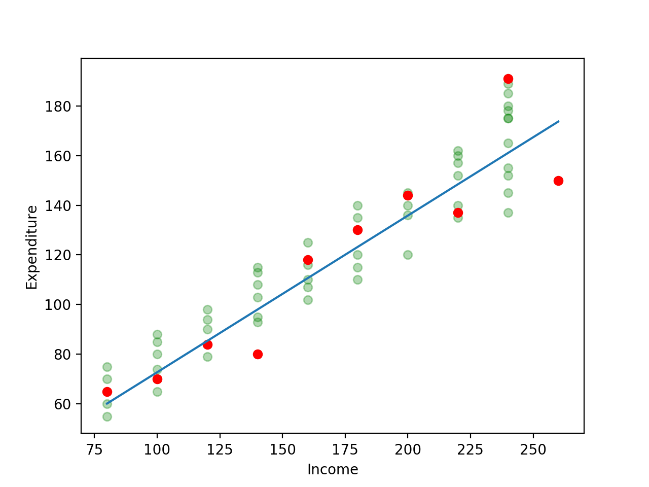
Let’s plot the line we obtained as a result of this.

Interpreting the Results

Our calculations gave us the results that and . Having a slope () of means that for every unit increase in income, there’s an increase of in expenditure. The intercept is where the regression line meets the Y axis. This means that even without any income, a persion would have an expenditure of . In a lot of cases, however, the intercept term doesn’t really matter as much as the slope and how to interpret the intercept depends upon what the Y axis represents.

Conclusion

That’s it for this post on bivariate linear regression. We saw how to calculate and and worked on a sample problem. We also saw how to interpret the result of the calculations. In the coming post we’ll look at how to assess whether the regression line is a good fit.

---

[1] It’s important to not confuse the stochastic error term with the residual . The stochastic error term represents the inherent variability of data whereas the residual represents the difference between the predicted and actual values of .