In the first part we saw the overall design of the system. In the second part we created a dataset that we can work with. In this post we’ll look at the first category of components and these are the ones that bring the data into the platform. We’ll see how we can stream data from the database using Debezium and store it in Pinot realtime tables.

Before we begin

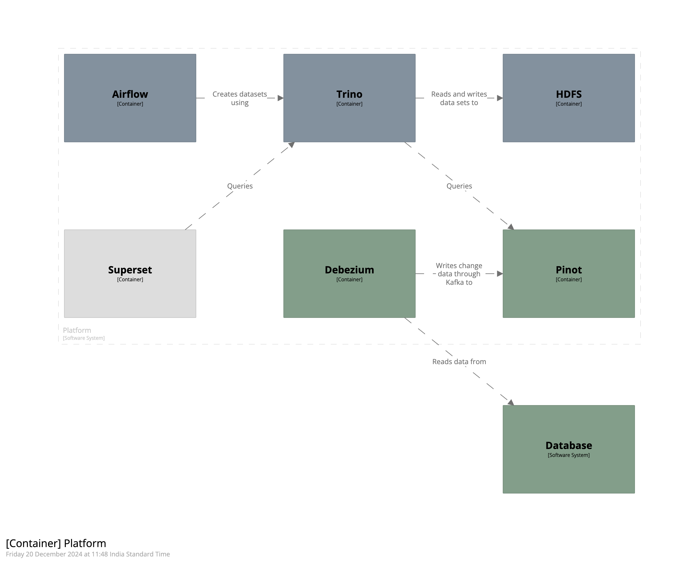
The setup is still Dockerized and now has containers for Debezium, Kafka, and Pinot. In a nutshell, we’ll stream data from the Postgres instance into Kafka using Debezium and then write it to Pinot tables.

Getting started

In the first part of the series we briefly looked at Debezium. To recap, Debezium is a platform for change data capture. It consists of connectors which capture change data from the database and emit them as events into Kafka. Which database tables to monitor and which Kafka topic to write them to are specified as a part of the connector’s configuration. This configuration is written as a JSON object and sent to a specfic endpoint to spawn a new connector.

We’ll begin by creating configuration for a connector which will monitor all the tables in the database and route each of them to a dedicated Kafka topic.

1
2
3
4
5
6
7
8
9
10
11
12
13
14
15
16
17
18
19
20
21
22
23
24
25
26

{
    "name": "order_service",
    "config": {
        "connector.class": "io.debezium.connector.postgresql.PostgresConnector",
        "database.hostname": "db",
        "database.user": "postgres",
        "database.password": "my-secret-pw",
        "database.dbname": "postgres",
        "database.server.name": "postgres",
        "plugin.name": "pgoutput",
        "publication.autocreate.mode": "filtered",
        "time.precision.mode": "connect",
        "tombstones.on.delete": "false",
        "snapshot.mode": "no_data",
        "heartbeat.interval.ms": "1000",
        "transforms": "route",
        "transforms.route.type": "org.apache.kafka.connect.transforms.RegexRouter",
        "transforms.route.regex": "([^.]+)\\.([^.]+)\\.([^.]+)",
        "transforms.route.replacement": "$3",
        "event.processing.failure.handling.mode": "skip",
        "producer.override.compression.type": "snappy",
        "signal.data.collection": "debezium.signal",
        "topic.prefix": "microservice",
        "decimal.handling.mode": "float"
    }
}

There are two main parts to this configuration - name and config. The name is the name we’ve given to the connector. The config contains the actual configuration of the connector. We specify quite a few things in the config object. We specify the class of the connector which is the fully qualified name of the Java class, the credentials to connect to the database, whether or not to take a snapshot, how to route the data to the appropriate Kafka topics, and how to pass signals to Debezium.

While most of the configuration is self-explanatory, we’ll look closely at the ones related to snapshot, signalling, and routing. We set the snapshot mode to no_data which means that the connector will stream historical rows from the database. The only rows that will be emitted are the ones created or updated after the connector began running. We’ll use this setting in conjunction with signals to incrementally snapshot the tables we’re interested in. Signals are a way to modify the behavior of the connector, or to trigger a one-time action like taking an ad-hoc snapshot. When we combine no_data with signals, we can tell Debezium to selectively snapshot the tables we’re interested in. The signal.data.collection property specifies the name of the table which the connector will monitor for any signals that are sent to it.

Finally, we specify a route transform. We do this by writing a regex which matches against the fully qualified name of the table, and extracts only the table name. This allows us to send the data from every table into a dedicated Kafka topic of its own.

Notice how we’ve not specified which tables to monitor. Since it is a Postgres database, the connector will monitor all the tables in all the schemas within the database and stream them. Now that the configuration is created, we’ll POST it to the appropriate endpoint to create the connector.

1

curl -H "Content-Type: application/json" -XPOST -d @tables/002-orders/debezium.json localhost:8083/connectors | jq .

Now that the connector is created, we will signal it to initiate a snapshot. Signals are sent to the connector using rows inserted into the table. We’ll execute the following INSERT query to tell the connector to take a snapshot of the orders table.

1
2
3
4
5
6

INSERT INTO debezium.signal 
VALUES (
    gen_random_uuid()::TEXT,
    'execute-snapshot',
    '{"data-collections": [".*\\.orders"], "type": "incremental"}'
);

The row tells the connector to initiate a snapshot, as indicated by execute-snapshot, and stream historical rows from the orders table in all the schemas within the database. It is an incremental snapshot so it will happen in batches. If we docker exec into the Kafka container and use the console consumer, we’ll find that all the rows eventually get streamed to the topic. The command to show it is given below.

1
2

[kafka@kafka ~]$ kafka-console-consumer.sh --bootstrap-server kafka:9092 --topic orders --from-beginning | wc -l
^CProcessed a total of 5000 messages

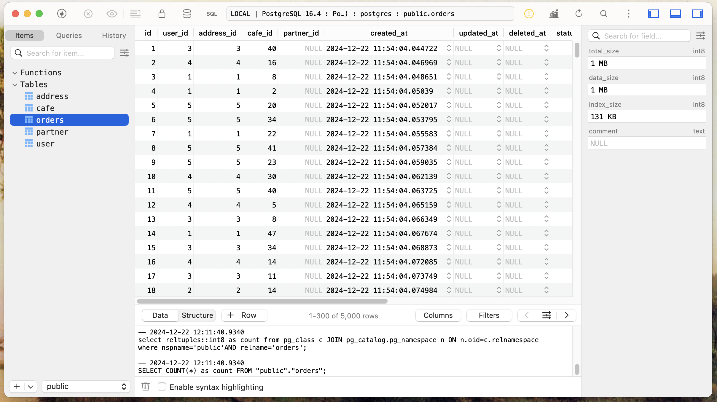
We can compare this with the row count in the table using the following SQL command.

1
2
3
4

SELECT COUNT(*) FROM public.orders;
| count |
|-------|
|  5000 |

Now that the data is in Kafka, we’ll move on to how to stream it into a Pinot table. Before we get to that, we’ll look at what a table and schema are in Pinot.

A table in Pinot is similar to a table in a relational database. It has rows and columns where each column has a datatype. Tables are where data is stored in Pinot. Every table in Pinot has an associated schema and it is in the schema where the columns and their datatypes are defined. Tables can be realtime, where they store data from a streaming source such as Kafka. They can be offline, where they load data from batch sources. Or they can be hybrid, where they load data from both a batch source and a streaming source. Both the schema and table are defined as JSON.

Let’s start by creating the schema.

1
2
3
4
5
6
7
8
9
10
11
12
13
14
15
16
17
18
19
20
21
22
23
24
25
26

{
  "schemaName": "orders",
  "enableColumnBasedNullHandling": true,
  "dimensionFieldSpecs": [
    {
      "name": "id",
      "dataType": "STRING"
    },
    {
      "name": "source",
      "dataType": "JSON"
    }
  ],
  "dateTimeFieldSpecs": [
    {
      "name": "created_at",
      "dataType": "LONG",
      "format": "1:MILLISECONDS:EPOCH",
      "granularity": "1:MILLISECONDS"
    }
  ],
  "primaryKeyColumns": [
    "id"
  ],
  "metricFieldSpecs": []
}

The schema defines a few things. It defines the name of the schema. This will also become the name of the table. Next, it defines the fields that will be present in the table. We’ve defined id, source, and created_at. The first two are specified in dimensionFieldSpecs and specify a column which becomes a dimension for any metric. The created_at field is specified in dateTimeFieldSpecs since it specifies a time column; Debezium will send timestamp columns as milliseconds since epoch. We’ve specified id as the primary key. Finally, enableColumnBasedNullHandling allows columns to have null values in them.

Once the schema is defined, we can create the table configuration.

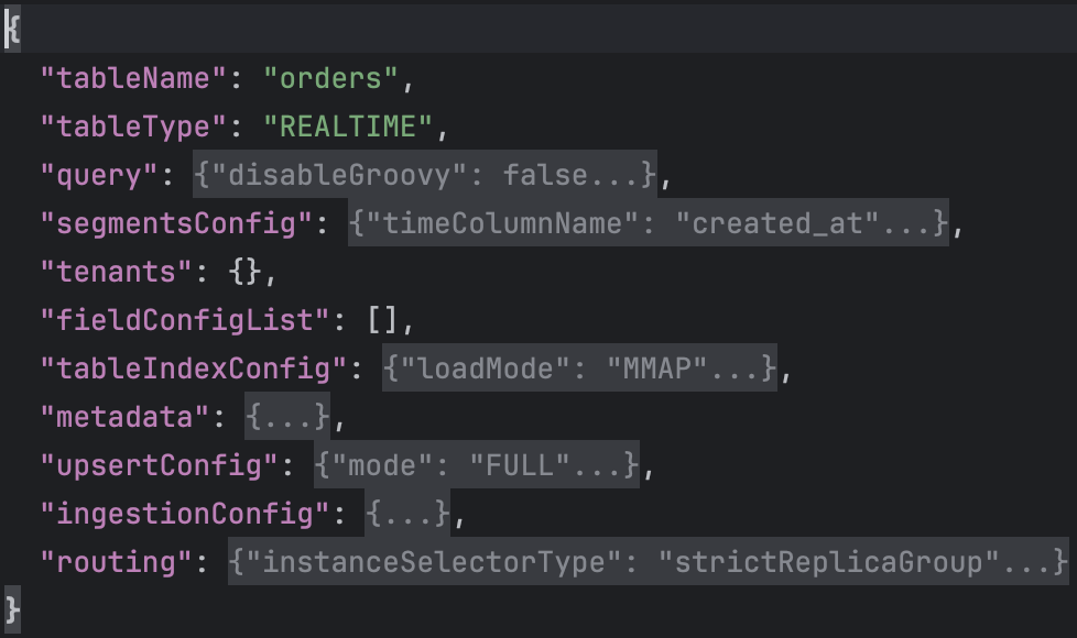
The configuration of tbe table is more involved than the schema so we’ll go over it one key at a time. We begin by specifying the tableName as “orders”. This matches the name of the schema. We specify tableType as “REALTIME” since the data we’re going to ingest comes from a Kafka topic. The query key specifies properties related to query execution. The segmentsConfig key specifies properties related to segments like the time column to use for creating a segment. The tenants key specifies the tenants for this table. A tenant is a logical namespace which restricts where the cluster processes queries on the table. The tableIndexConfig defines the indexing related information for the table. The metadata key specifies the metadata for this table. The upsertCconfig key specifies configuration for upserting into the table. The ingestionConfig key defines where we’d be ingesting data from and what field-level transformations we’d like to apply. The routing key defines properties that determine how the broker selects the servers to route.

The part of the configuration we’ll specifically look at is the ingestionConfig and upsertConfig. First, ingestionConfig.

1
2
3
4
5
6
7
8
9
10
11
12
13
14
15
16
17
18
19
20
21
22
23
24
25
26
27
28
29
30
31
32
33
34
35
36
37

{
  "ingestionConfig": {
    "streamIngestionConfig": {
      "streamConfigMaps": [
        {
          "realtime.segment.flush.threshold.rows": "0",
          "stream.kafka.decoder.prop.format": "JSON",
          "key.serializer": "org.apache.kafka.common.serialization.ByteArraySerializer",
          "stream.kafka.decoder.class.name": "org.apache.pinot.plugin.stream.kafka.KafkaJSONMessageDecoder",
          "streamType": "kafka",
          "value.serializer": "org.apache.kafka.common.serialization.ByteArraySerializer",
          "stream.kafka.consumer.type": "LOWLEVEL",
          "realtime.segment.flush.threshold.segment.rows": "50000",
          "stream.kafka.broker.list": "kafka:9092",
          "realtime.segment.flush.threshold.time": "3600000",
          "stream.kafka.consumer.factory.class.name": "org.apache.pinot.plugin.stream.kafka20.KafkaConsumerFactory",
          "stream.kafka.consumer.prop.auto.offset.reset": "smallest",
          "stream.kafka.topic.name": "orders"
        }
      ]
    },
    "transformConfigs": [
      {
        "columnName": "id",
        "transformFunction": "jsonPath(payload, '$.after.id')"
      },
      {
        "columnName": "source",
        "transformFunction": "jsonPath(payload, '$.after')"
      },
      {
        "columnName": "created_at",
        "transformFunction": "jsonPath(payload, '$.after.created_at')"
      }
    ]
  }
}

In the ingestionConfig we specify the the Kafka topics to read from. In the snippet above, we’ve specified the “orders” topic. We also specify field-level transformations in transformConfigs. Here we extract the id, source, and created_at fields from the JSON payload generated by Debezium.

With the schema and table defined, we’ll POST them to the appropriate endpoints using curl. The following two commands create the schema followed by the table.

1
2

curl -F schemaName=@tables/002-orders/orders_schema.json localhost:9000/schemas | jq .
curl -XPOST -H 'Content-Type: application/json' -d @tables/002-orders/orders_table.json localhost:9000/tables | jq .

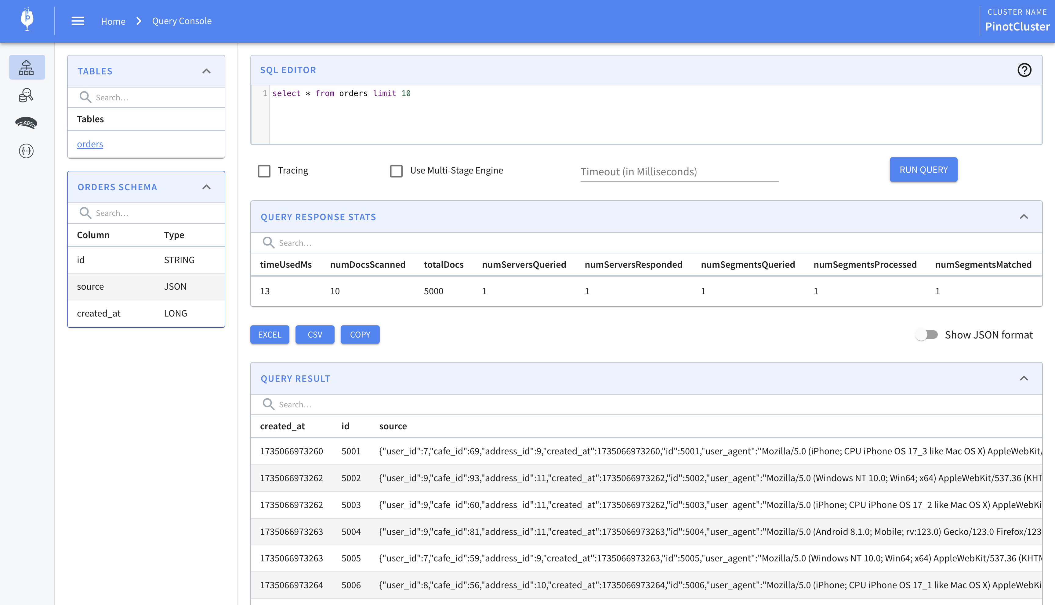
Once the table is created, it will begin ingesting data from the “orders” Kafka topic. We can view this data by opening the Pinot query console. Notice how the source column contains the entire “after” payload generated by Debezium.

That’s it. That’s how to stream data using Debezium into Pinot.

In the previous post we saw the overall design of the platform. We saw how the components of the system are divided into three separate categories: those that bring the data in, those that create datasets on this data, and those that display visualizations. Starting from this post, we’re going to start building the system. We’ll work with the data of a fictitious online cafe that we’ll populate using a Python script. In subsequent posts, we’ll ingest this data into the platform and create visualizations on top of it.

Before we begin

The setup, for this post, consists of a Docker container for Postgres which is a part of the compose file. We’ll bring up the container before we begin populating the database.

The data

We’ll create and populate a table which stores the orders placed by the customer. The table contains, among other fields, the id of the user who placed the order, the id of the address where the order needs to be delivered, the status of the order, and the user agent of the device used to place the order. The code snippet below shows how the model is represented as a Python class.

1
2
3
4
5
6
7
8
9
10
11
12
13
14
15
16
17

class Order(peewee.Model):
    """An order placed by the customer."""

    class Meta:
        table_name = "orders"
        database = database

    id = peewee.BigAutoField()
    user_id = peewee.IntegerField()
    address_id = peewee.IntegerField()
    cafe_id = peewee.IntegerField()
    partner_id = peewee.IntegerField(null=True)
    created_at = peewee.DateTimeField(default=datetime.datetime.now)
    updated_at = peewee.DateTimeField(null=True)
    deleted_at = peewee.DateTimeField(null=True)
    status = peewee.IntegerField(default=0)
    user_agent = peewee.TextField()

Once we’ve created this class, we’ll write a function which creates instances of this class and persists them in the database. There are classes representing the cafe, the addresses saved by the user, and the delivery partner who will be assigned to deliver the order. However, these have been left out for the sake of brevity. The code snippet below shows this function.

1
2
3
4
5
6
7
8
9
10
11
12
13
14
15
16
17
18
19
20
21
22
23
24
25
26
27
28
29

def create_orders(
    users: list[User],
    addresses: list[Address],
    cafes: list[Cafe],
    partners: list[Partner],
    n: int = 100,
) -> list[Order]:
    ua = UserAgent()
    orders = []

    def base_order() -> dict:
        cafe = cafes[random.randint(0, len(cafes) - 1)]
        user = users[random.randint(0, len(users) - 1)]
        addr = [_ for _ in addresses if _.user_id == user.id][0]
        user_agent = ua.random

        return {
            "user_id": user.id,
            "address_id": addr.id,
            "cafe_id": cafe.id,
            "user_agent": user_agent,
        }

    for _ in range(n):
        data = {**base_order(), "status": OrderStatus.PLACED.value}
        order = Order.create(**data)
        orders.append(order)

    return orders

Once we have all our classes and functions in place, we’ll run the script which populates the data.

1

python faker/data.py

We can now query the database to see our data.

This is it for the second part of the series.

I’d previously written about creating a data platform using Pinot, Trino, Airflow, and Debezium. It was a quick how-to that showed how to glue the pieces together to create a data platform. In this post we’ll go deeper into the design of the system and look at building the system in the posts that follow.

The design

A common requirement for data engineering teams is to move data stored within the databases owned by various microservices into a central data warehouse. One of the ways to move this data is by loading it incrementally. In this approach, once the data has been loaded fully, subsequent loads are done in smaller increments. These contain rows that have changed since the last time the warehouse was loaded. This brings the data into the warehouse periodically as the loads are run on a specified schedule.

Recently the shift has been towards moving data in realtime so that analytics can be derived quickly. Change data capture allows capturing row-level changes as they happen as a result of inserts, updates, and deletes in the tables. Responding to these events allows us to load the warehouse in realtime.

The diagram below shows how we can combine Pinot, Trino, Airflow, Debezium, and Superset to create a realtime data platform.

The components of the system can be divided into three broad categories. The first category is those that bring data into the platform and are shown in dark green. This category consists of the source database system, Debezium, and Pinot. Debezium reads the stream of changes happening in the database and writes them into Pinot. The second category is those that create datasets on top of the data ingested into Pinot and are shown in dark grey. This category consists of Airflow, Trino, and HDFS. Airflow uses Trino to create tables and views in HDFS on top of the data stored in Pinot. Finally, the last category is those that consume the datasets and present them to the end user. This category consists of data visualization tools like Superset.

Let’s discuss each of these components in more detail.

Debezium is a platform for change data capture. It consists of connectors which monitor the database tables for inserts, updates, and deletes and emit events into Kafka. These events can then be written into the data warehouse to create an up-to-date version of the table in the upstream database. We’ll run Debezium as a Docker container. When run like this, the connectors are available as a part of the image and can be configured using a REST API. To configure the connector we’ll send a JSON object to a specific endpoint. This object contains information such as the credentials of the database, the databases or tables we’d like to monitor, any transformations we’d like to apply to this data, and so on. As we’ll see when we begin building the system, we can monitor all of our tables for changes happening in them.

Pinot is an OLAP datastore that is built for real-time analytics. It supports creating tables that consume data in realtime so that insights can be derived quickly. Pinot, when combined with Debezium, allows us to ingest row-level changes as they happen in the source table. Configurations for Pinot tables and schemas are written in JSON and sent to their respective endpoints to create them. We’ll create a realtime table which ingests events emitted by Debezium. Using the upsert functionality provided by Pinot, we’ll keep only the latest state of the row in the table. This makes it easier to to create reports or do ad-hoc analysis.

Trino provides query federation by allowing us to query multiple data sources with a unified SQL interface. It is fast and distributed which means we can use it to query large amounts of data. We’ll use it in conjunction with Pinot since the latter does not yet provide full SQL capabilities. Trino allows connecting to a database by creating a catalog. As we can see from the diagram, we’ll need two catalogs - Pinot and HDFS. Since it is currently not possible to create views, materialized views, or tables from select statements in Pinot, we’ll create them in HDFS using Trino. This allows us to speed up the reports and dashboards since all of the required data will be precomputed and available in HDFS as either a materialized view or a table.

Airflow is an orchestrator that allows creating complex workflows. These workflows are created as Python scripts that define a directed acyclic graph (DAG) of tasks. Airflow then schedules these tasks for execution at defined intervals. Tasks are defined using operators. For example, to execute a Python function one would use the PythonOperator. Similarly, there are operators to execute SQL queries. We’ll use these operators to query Trino and create the datasets that are needed for reporting and dashboards. Peridocially regenerating these datasets would allow us to provide reports that present the latest data.

Superset is a data visualization tool. We’ll connect Superset to Trino so that we can visualize the datasets that we’ve created in HDFS.

Having discussed the various components of the design, let’s look at the design goals it achieves. First, the system is designed to be realtime. With change data capture using Debezium, we can respond to every insert, update, and delete happening in the source table as soon as it happens. Second, the system is designed with open-source technologies. This allows us to benefit from the experience of the collaborators and community behind each of these projects. Finally, the system is designed to be as close to self-service as possible. As we’ll see, the design of the system reduces the dependency of the of the downstream business analytics and data scientist teams on the data engineering team significantly.

This is it for the first part of the series.

I’d previously written about property-based testing in Clojure. In this blog post I’d like to talk about how we can do the same in Python using the Hypothesis library. We’ll begin with a quick recap of what property-based testing is, and then dive head-first into writing some tests.

What is property-based testing?

Before we get into property-based testing, let’s talk about how we usually write tests. We provide a known input to the code under test, capture the resulting output, and write an assertion to check that it matches our expectations. This technique of writing tests is called example-based testing since we provide examples of inputs that the code has to work with.

While this technique works, there are some drawbacks to it. Example-based tests take longer to write since we need to come up with examples ourselves. Also, it’s possible to miss out on corner cases.

In contrast, property-based testing allows us to specify the properties of the code and test that they hold true under a wide range of inputs. For example, if we have a function f that takes an integer and performs some computation on it, a property-based test would test it for positive integers, negative integers, very large integers, and so on. These inputs are generated for us by the testing framework and we simply need to specify what kind of inputs we’re looking for.

Having briefly discussed what property-based testing is, let’s write some code.

Writing property-based tests

Testing a pure function

Let’s start with a function which computes the n’th Fibonacci number.

1
2
3
4
5
6
7
8
9

@functools.cache
def fibonacci(n: int) -> int:
    """
    Computes the nth number in the Fibonacci sequence.
    """
    if n <= 1:
        return n

    return fibonacci(n - 1) + fibonacci(n - 2)

The sequence of numbers goes 0, 1, 1, 2, 3, etc. We can see that all of these numbers are greater than or equal to zero. Let’s write a property-based test to formalize this.

1
2
3
4
5
6
7

from hypothesis import given, strategies as st
from functions import fibonacci


@given(st.integers())
def test_fibonacci(n):
    assert fibonacci(n) >= 0

In the code snippet above, we’ve wrapped our test using the @given decorator. This makes it a property-based test. The argument to the decorator is a search strategy. A search strategy generates random data of a given type for us. Here we’ve specified that we need integers. We can now run the test using pytest as follows.

1

PYTHONPATH=. pytest .

The test fails with the following summary.

1

FAILED test/functions/test_fibonacci.py::test_fibonacci - ExceptionGroup: Hypothesis found 2 distinct failures. (2 sub-exceptions)

When looking at the logs, we find that the first failure is because the maximum recursion depth is reached when the value of n is large.

1
2
3

n = 453
... lines omitted ...
RecursionError: maximum recursion depth exceeded

The second failure is because the function returned a negative integer when the value of n is negative; in this case it is n=-1. This violates our assertion that the numbers in the Fibonacci sequence are non-negative.

1
2
3
4
5
6
7
8
9
10

+---------------- 2 ----------------
| Traceback (most recent call last):
|   File "/Users/fasih/Personal/pytesting/test/functions/test_fibonacci.py", line 8, in test_fibonacci
|     assert fibonacci(n) >= 0
| AssertionError: assert -1 >= 0
|  +  where -1 = fibonacci(-1)
| Falsifying example: test_fibonacci(
|     n=-1,
| )
+------------------------------------

To remedy the two failures above, we’ll add an assertion at the top of the function which will ensure that the input n is in some specified range. The updated function is given below.

1
2
3
4
5
6
7
8
9
10
11

@functools.cache
def fibonacci(n: int) -> int:
    """
    Computes the nth number in the Fibonacci sequence.
    """
    assert 0 <= n <= 300, f"n must be between 0 and 300; {n} was passed."

    if n <= 1:
        return n

    return fibonacci(n - 1) + fibonacci(n - 2)

We’ll update our test cases to reflect this change in code. The first test case checks the function when n is between 0 and 300.

1
2
3

@given(st.integers(min_value=0, max_value=300))
def test_fibonacci(n):
    assert fibonacci(n) >= 0

The second case checks when n is large. In this case we check that the function raises an AssertionError.

1
2
3
4

@given(st.integers(min_value=5000))
def test_fibonacci_large_n(n):
    with pytest.raises(AssertionError):
        fibonacci(n)

Finally, we’ll check the function with negative values of n. Similar to the previous test case, we’ll check that the function raises an AssertionError.

1
2
3
4

@given(st.integers(min_value=-2, max_value=-1))
def test_fibonacci_negative(n):
    with pytest.raises(AssertionError):
        fibonacci(n)

Testing persistent data

We’ll now use Hypothesis to generate data that we’d like to persist in the database. The snippet below shows a Person model with fields to store name and date of birth. The age property returns the current age of the person in years, and the MAX_AGE variable indicates that the maximum age we’d like to allow in the system is 120 years.

1
2
3
4
5
6
7
8
9
10
11
12
13
14

class Person(peewee.Model):

    MAX_AGE = 120

    class Meta:
        database = db

    id = peewee.BigAutoField(primary_key=True, null=False)
    name = peewee.CharField(null=False, max_length=120)
    dob = peewee.DateField(null=False)

    @property
    def age(self) -> int:
        return (datetime.date.today()).year - self.dob.year

We’ll add a helper function to create Person instances as follows.

1
2
3
4
5
6
7
8
9

def create(name: str, dob: datetime.date) -> Person:
    """
    Create a new person instance with the given name and date of birth.
    :param name: Name of the person.
    :param dob: Date of birth of the person.
    :return: A Person instance.
    """
    assert name, f"name cannot by empty"
    return Person.create(name=name, dob=dob)

Like we did for the function which computes Fibonacci numbers, we’ll add a test case to formalize this expectation. This time we’re generating random names and dates of birth and passing them to the helper function.

1
2
3
4
5
6
7

@given(
    text=st.text(min_size=1),
    dob=st.dates(),
)
def test_create_person(text, dob, create_tables):
    person = pr.create(name=text, dob=dob)
    assert 0 <= person.age <= Person.MAX_AGE

I’m persisting this data in a Postgres table and the create_tables fixture ensures that the tables are created before the test runs.

Upon running the test we find that it fails for two cases. The first case is when the input string contains a NULL character \x00. Postgres tables do not allow strings will NULL characters in them.

1
2
3
4
5
6

ValueError: A string literal cannot contain NUL (0x00) characters.
Falsifying example: test_create_person(
     create_tables=None,
     text='\x00',
     dob=datetime.date(2000, 1, 1),  # or any other generated value
)

The second case is when the date of birth is in the future.

1
2
3
4
5
6
7

AssertionError: assert 0 <= -1
  +  where -1 = <Person: 5375>.age
 Falsifying example: test_create_person(
     create_tables=None,
     text='0',  # or any other generated value
     dob=datetime.date(2025, 1, 1),
)

To remedy the first failure, we’ll have to sanitize the name input string that gets stored in the table. We’ll create a helper function which removes any NULL characters from the string. This will be called before name gets saved in the table.

1
2

def sanitize(s: str) -> str:
    return s.replace("\x00", "").strip()

To remedy the second failure, we’ll add an assertion ensuring that the age is less than or equal to 120. The updated create function is shown below.

1
2
3
4
5
6
7
8
9
10
11
12
13

def create(name: str, dob: datetime.date) -> Person:
    """
    Create a new person instance with the given name and date of birth.
    :param name: Name of the person.
    :param dob: Date of birth of the person.
    :return: A Person instance.
    """
    name = sanitize(name)

    assert name, f"name cannot by empty"
    assert 0 <= (datetime.date.today().year - dob.year) <= Person.MAX_AGE

    return Person.create(name=name, dob=dob)

We’ll update the test cases to reflect these changes. Let’s start by creating two variables that will hold the minimum and maximum dates allowed.

1
2

MIN_DATE = datetime.date.today() - datetime.timedelta(days=Person.MAX_AGE * 365)
MAX_DATE = datetime.date.today()

Next, we’ll add a test to ensure that we raise an AssertionError when the string contains only NULL characters.

1
2
3
4

@given(text=st.text(alphabet=["\x00"]))
def test_create_person_null_text(text, create_tables):
    with pytest.raises(AssertionError):
        pr.create(name=text, dob=MIN_DATE)

Next, we’ll add a test to ensure that dates cannot be in the future.

1
2
3
4
5
6
7

@given(
    text=st.text(min_size=1),
    dob=st.dates(min_value=MAX_DATE + datetime.timedelta(days=365)),
)
def test_create_person_future_dob(text, dob, create_tables):
    with pytest.raises(AssertionError):
        pr.create(name=text, dob=dob)

Similarly, we’ll add a test to ensure that dates cannot be more than 120 years in the past.

1
2
3
4
5
6
7

@given(
    text=st.text(min_size=1),
    dob=st.dates(max_value=MIN_DATE - datetime.timedelta(days=365)),
)
def test_create_person_past_dob(text, dob, create_tables):
    with pytest.raises(AssertionError):
        pr.create(name=text, dob=dob)

Finally, we’ll add a test to ensure that in all other cases, the function creates a Person instance as expected.

1
2
3
4
5
6
7
8
9
10

@given(
    text=st.text(min_size=5),
    dob=st.dates(
        min_value=MIN_DATE,
        max_value=MAX_DATE,
    ),
)
def test_create_person(text, dob, create_tables):
    person = pr.create(name=text, dob=dob)
    assert 0 <= person.age <= Person.MAX_AGE

The tests pass when we rerun them so we can be sure that the function behaves as expected.

Testing a REST API.

Finally, we’ll look at testing a REST API. We’ll create a small Flask app with an endpoint which allows us to create Person instances. The API endpoint is a simple wrapper around the create helper function and returns the created Person instance as a dictionary.

1
2
3
4
5
6
7
8
9
10

@api.route("/person", methods=["POST"])
def create_person():
    name = request.json["name"]

    dob = request.json["dob"]
    dob = parse(dob).date()

    person = pr.create(name, dob)

    return model_to_dict(person)

We’ll add a test to generate random JSON dictionaries which we’ll pass as the body of the POST request. The test is given below.

1
2
3
4
5
6
7
8
9
10
11
12
13
14
15
16

@given(
    json=st.fixed_dictionaries(
        {
            "name": st.text(min_size=5),
            "dob": st.dates(min_value=MIN_DATE, max_value=MAX_DATE),
        }
    )
)
def test_create_person(json, test_client):
    response = test_client.post(
        "/api/person",
        json=json,
        headers={"Content-Type": "application/json"},
    )

    assert response.status_code == 200

Similar to the tests for create function, we test that the API returns a response successfully when the inputs are proper.

That’s it. That’s how we can leverage Hypothesis to test Python code. You’ll find the code for this post in the Github repository.

In the previous post we looked at computing the Fibonacci series both with and without dynamic programming. In this post we’ll look at another example where dynamic programming is applicable. The example is borrowed from ‘Introduction to Algorithms’ by CLRS and implemented in Python. By the end of this post we’ll try to develop an intuition for when dynamic programming applies.

Rod Cutting

The problem we are presented with is the following: given a steel rod, we’d like to find the optimal way to cut it into smaller rods. More formally, we’re presented with a rod of size n inches and a table of prices p_i. We’d like to determine the maximum revenue r_n that we can obtain by cutting the rod and selling it. If the price p_n of the rod of length n is large enough, we may sell the rod without making any cuts.

The table of prices that we’ll work with is given below.

Consider a rod of length 4 inches. The maxium revenue we can obtain is 10 by cutting the rod into two parts of length 2 inches each.

Given a rod of n inches, we may sell it uncut or we may sell it by cutting it into smaller pieces. Since we do not know the size of the cuts to make, we will have to consider all possible sizes. Once we make a cut of size from the left end of the rod, we can view the remaining length of the rod of size as an independent instance of the rod cutting problem. In other words, we are solving a smaller instance of the same problem. The equation below shows how we can mathematically formulate the problem.

It states that the revenue r_n is the maximum revenue obtained by considering all cuts of size plus the revenue obtained by cutting the remaining rod of size . We can write a recursive function to obtain this value as follows:

1
2
3
4
5
6
7
8
9
10

def rod_cut(p: list[int], n: int) -> int:
    if n == 0:
        return 0

    q = float("-inf")

    for i in range(1, n + 1):
        q = max(q, p[i] + rod_cut(p, n - i))

    return q

We can verify the results by calling the function for a rod of size 4 and passing the table of prices.

1
2

p = [0, 1, 5, 8, 9, 10, 17, 17, 20, 24, 30]
assert 10 == rod_cut(p=p, n=4)

The recursive version, however, does redundant work. Consider the rod of size n = 4. We will have to consider cuts of size . When considering the remaining rod of size 3, we’d consider cuts of size . In both of these cases we recompute, for example, the revenue obtained when the remainder of the rod is of size 2.

We can use dynamic programming to solve this problem by modifying the rod_cut function as follows.

1
2
3
4
5
6
7
8
9
10
11
12
13
14
15

def rod_cut(p: list[int], t: list[int | None], n: int) -> int:
    if n == 0:
        return 0

    if t[n] is not None:
        return t[n]

    q = float("-inf")

    for i in range(1, n + 1):
        q = max(q, p[i] + rod_cut(p, t, n - i))

    t[n] = q

    return q

Notice how we’ve introduced a table t which stores the maximum revenue obtained by cutting a rod of size n. This allows us to reuse previous computations. We can run this function and verify the result.

1
2
3

t = [None] * 11
p = [0, 1, 5, 8, 9, 10, 17, 17, 20, 24, 30]
assert 10 == rod_cut(p, t, 4)

The question that we’re left with is the following: how did we decide that the problem could be solved with dynamic programming? There are two key factors that help us in deciding if dynamic programming can be used. The first is overlapping subproblems and the second is optimal substructure.

For a dynamic programming algorithm to work, the number of subproblems must be small. This means that the recursive algorithm which solves the problem encounters the same subproblems over and over again. When this happens, we say that the problem we’re trying to solve has overlapping subproblems. In the rod cutting problem, when we try to cut a rod of size 4, we consider cuts of size . When we, then, consider the remaining rod of size 3, we consider cuts of size . The smaller problem of optimally cutting the rod of size 2 is encountered again. In other words, it is an overlapping subproblem. Dynamic programming algorithms solve an overlapping subproblem once and store its result in a table so that it can be reused again.

The second factor is optimal substructure. When a problem exhibits optimal substructure, it means that the solution to the problem contains within it the optimal solutions to the subproblems; we build an optimal solution to the problem from optimal solutions to the subproblems. The rod-cutting problem exhibits optimal substructure because the optimal solution to cutting a rod of length involves finding the optimal solution to cutting the remaining rod, if a cut has been made.

Moving on. So far our algorithm has returned the optimal value of the solution. In other words, it returned the maximum revenue that can be obtained by optimaly cutting the rod. We often need to store the choice that led to the optimal solution. In the context of the rod cutting problem, this would be the lengths of the cuts made. We can do this by keeping additional information in a separate table. The following code listing is a modification of the above function with an additional table s to store the value of the optimal cut.

1
2
3
4
5
6
7
8
9
10
11
12
13
14
15
16
17
18
19
20
21

def rod_cut(p: list[int], s: list[int | None], t: list[int | None], n: int) -> int:
    if n == 0:
        return 0

    if t[n] is not None:
        return t[n]

    q = float("-inf")
    j = None

    for i in range(1, n + 1):
        r = p[i] + rod_cut(p, s, t, n - i)

        if r > q:
            q = r
            j = i

    s[n] = j
    t[n] = q

    return q

In this version of the code, we store the size of the cut being made for a rod of length n in the table s. Once we have this information, we can reconstruct the optimal solution. The function that follows shows how to do that.

1
2
3
4
5
6
7
8
9

def optimal_cuts(s: list[int | None], n: int) -> list[int]:
    cuts = []

    while n:
        cut = s[n]
        n = n - s[n]
        cuts.append(cut)

    return cuts

Finally, we call the function to see the optimal solution. Since we know that the optimal solution for a rod of size 4 is to cut it into two equal halves, we’ll use .

1
2
3
4
5
6
7

n = 4
t = [None] * 11
s = [None] * 11
p = [0, 1, 5, 8, 9, 10, 17, 17, 20, 24, 30]
q = rod_cut(p, s, t, n)

assert [2, 2] == optimal_cuts(s, n)

That’s it. That’s how we can use dynamic programming to optimally cut a rod of size inches.

In this post, and hopefully in the next few posts, I’d like to devle into the topic of dynamic programming. The aim is to develop an intuition for when it is applicable by solving a few puzzles. I’ll be referring to the chapter on dynamic programming in ‘Introduction to Algorithms’ by CLRS, and elucidating it in my own words.

Dynamic Programming

The chapter opens with the definition of dynamic programming: it is a technique for solving problems by combining solutions to subproblems. The subproblems may have subsubproblems that are common between them. A dynamic programming algorithm solves these subsubproblems only once and saves the result, thereby avoiding unnecessary work. The term “programming” refers to a tabular method in which the results of subsubproblems are saved in a table and reused when the same subsubproblem is encountered again.

All of this is abstract so let’s look at a concrete example of computing the Fibonacci series.

1
2

def fibonacci(n: int) -> int:
    return n if n < 2 else fibonacci(n - 1) + fibonacci(n - 2)

The call graph for fibonacci(4) is given below.

As we can see, we’re computing fibonacci(2) twice. In other words, the subsubproblem of computing fibonacci(2) is shared between fibonacci(4) and fibonacci(3). A dynamic programming algorithm would solve this subsubproblem only once and save the result in a table and reuse it. Let’s see what that looks like.

1
2
3
4
5
6
7
8
9

def fibonacci(n: int) -> int:
    T = [0, 1] + ([None] * (n - 2))
    return fibonacci_helper(n=n - 1, T=T)


def fibonacci_helper(n: int, T: list[int | None]) -> int:
    if T[n] is None:
        T[n] = fibonacci_helper(n - 1, T) + fibonacci_helper(n - 2, T)
    return T[n]

In the code above, we create a table T which stores the Fibonacci numbers. If an entry exists in the table, we return it immediately. Otherwise, we compute and store it. This recursive approach, with results of subsubproblems stored in a table, is called “top-down with memoziation”; the table is called the “memo”. We begin with the original problem and then proceed to solve it by finding solutions to smaller subproblems. The procedure which computes the solution is said to be “memoized” as it remembers the previous computations.

Another approach is called “bottom-up” in which the solutions to the smaller subproblems are computed first. This depends on the notion that subproblems have “size”. In this approach, a solution to the subproblem is found only when the solutions to its smaller subsubproblems have been found. We can apply this approach when computing the Fibonacci series.

1
2
3
4
5
6
7

def fibonacci(n: int) -> int:
    T = [0, 1] + ([None] * (n - 2))

    for i in range(2, n):
        T[i] = T[i - 1] + T[i - 2]

    return T[n - 1]

As we can see, the larger numbers in the Fibonacci series are computed only when the smaller numbers have been computed.

This was a small example of how dynamic programming algorithms work. They are applied to problems where subproblems share subsubproblems. The solutions to these subsubproblems are stored in a table and reused when they are encountered again. This enables the algorithm to work more efficiently as it avoids the rework of solving the subsubproblems.

In the next post we’ll look at another example of dynamic programming that’s presented in the book and implement it in Python to further our understanding of the subject.

I’d recently written about an experimental library to detect PII. When discussing it with an acquaintance of mine, I was told that PII can also be disguised. For example, a corpus of text like a review or a comment can contain email address in the form “johndoeatgmaildotcom”. This led me to update the library so that emails like these can also be flagged. In a nutshell, I had to update the regex which was used to find the email.

Example

This is best explained with a few examples. In all of the examples, we begin with a proper email and disguise it one step at a time.

1
2
3
4
5
6
7
8
9

column = Column(name="comment")
detector = ColumnValueRegexDetector()

assert detector.detect(column=column, sample="john.doe@provider.com") == Email()
assert detector.detect(column=column, sample="johndotdoe@provider.com") == Email()
assert detector.detect(column=column, sample="johndotdoeatproviderdotcom") == Email()
assert detector.detect(column=column, sample="john.doe@provider.co.uk") == Email()
assert detector.detect(column=column, sample="johndotdoeatproviderdotcodotuk") == Email()
assert detector.detect(column=column, sample="myemailis:john.doeatproviderdotcom") == Email()

All of these assertions pass and the regex detector is able to flag all of these examples as email.

I recently created an experimental library, detectpii, to detect PII data in relational databases. In this post we’ll take a look at the rationale behind the library and it’s architecture.

Rationale

A common requirement in many software systems is to store PII information. For example, a food ordering system may store the user’s name, address, phone number, and email. This information may also be replicated into the data warehouse. As a matter of good data governance, you may want to restrict access to such information. Many data warehouses allow applying a masking policy that makes it easier to redact such values. However, you’d have to specify which columns to apply this policy to. detectpii makes it easier to identify such tables and columns.

My journey into creating this library began by looking for open-source projects that would help identify such information. After some research, I did find a few projects that do this. The first project is piicatcher. It allows comparing the column names of tables against regular expressions that represent common PII column names like user_name. The second project is CommonRegex which allows comparing column values against regular expression patterns like emails, IP addresses, etc.

detectpii combines these two libraries to allow finding column names and values that may potentially contain PII. Out of the box, the library allows scanning column names and a subset of its values for potentially PII information.

Architecure

At the heart of the library is the PiiDetectionPipeline. A pipeline consists of a Catalog, which represents the database we’d like to scan, and a number of Scanners, which perform the actual scan. The library ships with two scanners - the MetadataScanner and the DataScanner. The first compares column names of the tables in the catalog against known patterns for the ones which store PII information. The second compares the value of each column of the table by retrieving a subset of the rows and comparing them against patterns for PII. The result of the scan is a list of column names that may potentially be PII.

The design of the library is extensible and more scanners can be added. For example, a scanner to use a proprietary machine learning algorithm instead of regular expression match.

Usage

To perform a scan, we create a pipeline and pass it a catalog and a list of scanners. To inititate the scan, we call the scan method on the pipeline to get back a list of PII columns.

1
2
3
4
5
6
7
8
9
10
11
12
13
14
15
16
17
18
19
20
21
22
23
24
25

from detectpii.catalog import PostgresCatalog
from detectpii.pipeline import PiiDetectionPipeline
from detectpii.scanner import DataScanner, MetadataScanner

# -- Create a catalog to connect to a database / warehouse
pg_catalog = PostgresCatalog(
    host="localhost",
    user="postgres",
    password="my-secret-pw",
    database="postgres",
    port=5432,
    schema="public"
)

# -- Create a pipeline to detect PII in the tables
pipeline = PiiDetectionPipeline(
    catalog=pg_catalog,
    scanners=[
        MetadataScanner(),
        DataScanner(percentage=20, times=2,),
    ]
)

# -- Scan for PII columns.
pii_columns = pipeline.scan()

That’s it. That’s how to use the library to detect PII columns in tables.

In the exercises that follow the chapter on algebraic manipulations, there is a question that pertains to expressing an integer as the sum of two other integers squared. We are then asked to find expressions for the multiples of , namely and . In this post, we’ll take a look at the solution provided by the authors for the first half of the question, , and then come up with a method of our own to solve the second half, .

Question

If is an integer that can be expressed as the sum of two integer squares, show that both and can also be expressed as the sum of two integer squares.

Solution

From the question, since it is the sum of two integer squares. This means . We need to find two integers such that when their squares are summed, we end with . From the solution, these are the numbers (a + b) and (a - b) because when they are squared and summed, we get . This is the result of . Go ahead and expand them to verify the result.

What do we deduce from this? We find that both the expressions contributed an and a . These were added together to get the final result. How do we use this to get ? Notice that we’re squaring the integers. This means that, for example, one of them would have to contribute an and the other would have to contribute a ; similar logic applies for .

This leaves us with two pairs of numbers — and . Let’s square and sum both of these numbers one-by-one.

What integers would we need for ?

In a previous post we’d seen how to create a realtime data platform with Pinot, Trino, Airflow, and Debezium. In this post we’ll see how to setup a data catalog using DataHub. A data catalog, as the name suggests, is an inventory of the data within the organization. Data catalogs make it easy to find the data within the organisation like tables, data sets, reports, etc.

Before we begin

My setup consists of Docker containers required to run DataHub. While DataHub provides features like data lineage, column assertions, and much more, we will look at three of the simpler featuers. One, we’ll look at creating a glossary of the terms that will be used frequently in the organization. Two, we’ll catalog the datasets and views that we saw in the previous post. Three, we’ll create an inventory of dashboards and reports created for various departments within the organisation.

The rationale for this as follows. Imagine a day in the life of a business analyst. Their responsibilities include creating reports and dashboards for various departments. For example, the marketing team may want to see an “orders by day” dashboard so that they can correlate the effects of advertising campaigns with an uptick in the volume of orders. Similarly, the product team may want a report of which features are being used by the users. The requests of both of these teams will be served by the business analyts using the data that’s been brought into the data platform. While they create these reports and dashboards, it’s common for them to receive queries asking where a team member can find a certain report or how to interpret a data point within a report. They may also have to search for tables and data sets to create new reports, acquaint themselves with the vocabulary of the various departments, and so on.

A data catalog makes all of this a more efficient process. In the following sections we’ll see how we can use DataHub to do it. For example, we’ll create the definition of the term “order”, create a list of reports created for the marketing department, and bring in the views and data sets so that they become searchable.

The work of data scientists is similar, too, because they create data sets that can be reused across various models. For example, data sets representing features for various customers can be stored in the platform, made searchable, and used with various models. They, too, benefit from having a data catalog.

Finally, it helps bring people up to speed with the data that is consumed by their department or team. For example, when someone joins the marketing team, pointing them to the data catalog helps them get productive quickly by finding the relevant reports, terminology, etc.

Ingesting data sets and views

To ingest the tables and views, we’ll create a data pipeline which ingets metadata from AWS Glue and writes it to the metadata service. This is done by creating a YAML configuration in DataHub that specifies where to ingest the metadata from, and where to write it. Once this is created, we can schedule it to run periodically so that it stays updated with Glue.

The image above shows how we define a “source” and how we ingest it into a “sink”. Here we’ve specified that we’d like to read from Glue and write it to DataHub’s metadata service.

Once the source and destination are defined, we can set a schedule to run the ingestion. This will bring in the metadata about the data sets and views we’ve created in Glue.

The image above shows that a successful run of the ingestion pipeline brings in the views and data sets. These are then browsable in the UI. Similarly, they are also searchable as shown in the following image.

This makes it possible for the analysts and the data scientists to quickly locate data sets.

Defining the vocabulary

Next, we’ll create the definition of the word “order”. This can be done from the UI as shown below. The definition can be added by editing the documentation.

Once created, this is available under “Glossary” and in search results.

Data products

Finally, we’ll create a data product. This is the catalog of reports and dashboards created for various departments. For example, the image below shows a dashboard created for the marketing team.

Expanding the dashboard allows us to look at the documentation for the report. This could contain the definition of the terms used in the report, as shown on the bottom right, a link to the dashboard in Superset, definitions of data points, report owners, and so on.

That’s it. That’s how a data catalog helps streamline working with data.

As I continue working my way through the book on programming puzzles, I came across those involving permutations. In this post I’ll collect puzzles with the same theme, both from the book and from the internet.

All permutations

The first puzzle is to compute all the permutations of a given array. By extension, it can be used to compute all the permutations of a string, too, if we view it as an array of characters. To do this we’ll implement Heap’s algorithm. The following is its recursive version.

1
2
3
4
5
6
7
8
9
10
11
12
13

def heap(permutations: list[list], A: list, n: int):
    if n == 1:
        permutations.append(list(A))
    else:
        heap(permutations, A, n - 1)

        for i in range(n - 1):
            if n % 2 == 0:
                A[i], A[n - 1] = A[n - 1], A[i]
            else:
                A[0], A[n - 1] = A[n - 1], A[0]

            heap(permutations, A, n - 1)

The array permutations is the accumulator which will store all the permutations of the array. The initial arguments to the function would be an empty acuumulator, the list to permute, and the length of the list.

Next permutation

The next puzzle we’ll look at is computing the next permutation of the array in lexicographical order. The following implementation has been taken from the book.

1
2
3
4
5
6
7
8
9
10
11
12
13
14
15
16
17

def next_permutation(perm: list[int]) -> list[int]:
    inversion_point = len(perm) - 2

    while (inversion_point >= 0) and (perm[inversion_point] >= perm[inversion_point + 1]):
        inversion_point = inversion_point - 1

    if inversion_point == -1:
        return []

    for i in reversed(range(inversion_point + 1, len(perm))):
        if perm[i] > perm[inversion_point]:
            perm[inversion_point], perm[i] = perm[i], perm[inversion_point]
            break

    perm[inversion_point + 1:] = reversed(perm[inversion_point + 1:])

    return perm

Previous permutation

A variation of the puzzle is to compute the previous permutation of the array in lexicographical order. The idea is to “reverse” the logic for computing the next permutation. If we look closely, we’ll find that all we’re changing are the comparison operators.

1
2
3
4
5
6
7
8
9
10
11
12
13
14
15
16
17

def previous_permutation(perm: list[int]) -> list[int]:
    inversion_point = len(perm) - 2

    while (inversion_point >= 0) and (perm[inversion_point] <= perm[inversion_point + 1]):
        inversion_point = inversion_point - 1

    if inversion_point == -1:
        return []

    for i in reversed(range(inversion_point + 1, len(perm))):
        if perm[i] < perm[inversion_point]:
            perm[inversion_point], perm[i] = perm[i], perm[inversion_point]
            break

    perm[inversion_point + 1:] = reversed(perm[inversion_point + 1:])

    return perm

kth smallest permutation

The final puzzle we’ll look at is the one where we need to compute the k’th smallest permutation. The solution to this uses the previous_permutation function that we saw above. The idea is to call this function k times on the lexicographically-largest array. Sorting the array in decreasing order results is the largest. This becomes the input to the previous_permutation function.

1
2
3
4
5
6
7
8
9

def kth_smallest_permutation(perm: list[int], k: int) -> list[int]:
    # -- Arrange the numbers in decreasing order
    # -- thereby creating the lexicographically largest permutation
    perm = sorted(perm, reverse=True)

    for _ in range(k):
        perm = previous_permutation(perm)

    return perm

That’s it. These are puzzles involving permutations.