The first topic we’ll look at is linear regression. As mentioned previously, regression is about understanding dependence of one variable on another. We’ll start by building an intuitive understanding of what it is before we dive into the math-y details of it. We’ll cover the theory, learn to solve some problems by hand, look at the assumptions supporting it, then look at what happens if these assumptions aren’t held. Once this is done we’ll look at how we can do the same by using gradient descent.
What is Regression Analysis?
Regression analysis is the study of the dependence of one variable (dependent variable, regressand) over one or more other variables (explanatory variables, regressors). The aim is to see how the dependent variable changes, on average, if there is a change in the explanatory variables. This is better explained with an example.
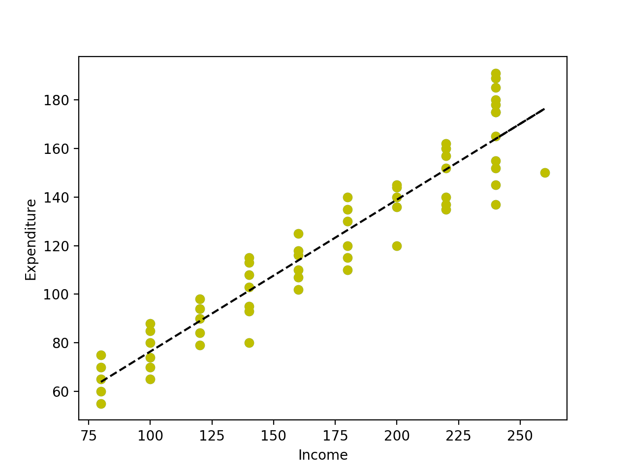
The plot shown here is of daily income and daily expenditure. The dependent variable here is the expenditure which depends on the explanatory variable income. As we can see from the plot, for every income level we have a range of expenditures. However, as the regression line shows, on average as income goes up, the expenditure goes up, too.
Why do we say that the income goes up on average? Let’s look at the raw data when daily income is 80 or 100.
1 | income (X) expenditure (Y) average |
The highest expenditure when income is 80 (75) is greater than the lowest expenditure when income level is 100 (65). If we look at the averages, the expenditure has gone up. There are a number of factors which may have caused the person with income 80 to expend 75 but as a whole, people with his daily income tend to expend less than those who earn 100 a day. The regression line passes through these averages.
That’s the basic idea behind regression analysis.
The Math behind Regression Analysis
The regression line passes through the average expenditure for every given income level. In other words, it passes through the conditional expected value —
We can start by assuming
Now given that we know how to calculate the average expenditure for a given income level, how do we calculate the expenditure of each individual at that income level? We can say that the individual’s expenditure is “off the average expenditure by a certain margin”. This can be written as
No matter how good our regression model is, there is always going to be some inherent variability. There are factors other than income which define a person’s expenditure. Factors like gender, age, etc. affect the expenditure. All of these factors are subsumed into the stochastic error term.
When it comes to applying regression analysis, we won’t have access to the population data. Rather, we have access to sample data. Our task is to come up with sample regression coefficients such that they’ll be as close as possible to the population regression coefficients. The sample regression function is defined as:
Here
What it means to be ‘Linear’
Linearity can be defined as being either linear in parameters or linear in explanatory variables. To be linear in parameters means that all your parameters in the regression function will have power 1. By that definition,
That’s it. This is what sets the foundation for further studying linear regression.