In the previous post we calculated the values of and from a given sample and in closing I mentioned that we’ll take a look at finding out whether the sample regression line we obtained is a good fit. In other words, we need to assess how close and are to and or how close is to . Recall that the population regression function (PRF) is given by . This shows that the value of depends on and . To be able to make any statistical inference about (and and ) we need to make assumptions about how the values of and were generated. We’ll discuss these assumptions in this post as they’re important for the valid interpretation of the regression estimates.
Classic Linear Regression Model (CLRM)
There are 7 assumptions that Gaussian or Classic linear regression model (CLRM) makes. These are:
1. The regression model is linear in parameters
Recall that the population regression function is given by . This is linear in parameters since and have power 1. The explanatory variables, however, do not have to be linear.
2. Values of X are fixed in repeated sampling
In this series of posts, we’ll be looking at fixed regressor models[1] where the values of X are considered to be fixed when drawing a random sample. For example, in the previous post the values of X were fixed between 80 and 260. If another sample were to be drawn, the sample values of X would be used.
3. Zero mean value of the error term
This assumption states that for every given , the error term is zero, on average. This should be intuitive. The regression line passes through the conditional mean for every . The error term are distances of the individual points from the conditional mean. Some of them lie above the regression line and some of them lie below. However, they cancel each other out; the positive cancel out the negative and therefore is zero, on average. Notationally, .
What this assumption means that all those variables that were not considered to be a part of the regression model do not systematically affect i.e. their effect on average is zero on .
This assumption also means is that there is no specification error or specification bias. This happens when we chose the wrong functional form for the regression model, exclude necessary explanatory variables or include unnecessary ones.
4. Constant variance of (homoscedasticity)
This assumption states that the variation of is the same regardless of .
With this assumption, we assume that the variance of for a given (i.e. conditional variance) is a positive constant value given by . This means that the variance for the various populations is the same. What this also means is that the variance around the regression line is the same and it neither increases nor decreases with change in values of .
5. No autocorrelation between disturbances
Given any two values, and (), the correlation between any two and is zero. In other words, the observations are independently sampled. Notationally, . This assumption states that there is no serial correlation or autocorrelation i.e. and are uncorrelated.
To build an intuition, let’s consider the population regression function
Now suppose that and are positively correlated. This means that depends not only on but also on because that affects . Autocorrelation occurs in timeseries data like stock market trends where the the observation of one day depends on the observation of the previous day. What we assume is that each observation is independent as it is in case of the income-expense example we saw.
6. The sample size must be greater than the number of parameters to estimate
This is fairly simple to understand. To be able to estimate and , we need atleast 2 pairs of observations.
7. Nature of X variables
There are a few things we assume about the value of variables. One, for a given sample they are not all the same i.e. is a positive number. Second, there are no outliers among the values.
If we have all the values of the same in a given sample, the regression line would be a horizontal line and therefore it will be impossible to estimate and thus . This will happen because in the equation , the denominator will become zero since and will be the same.
Furthermore, we assume that there are no outliers in the values. Suppose there are a few values which are far apart from the mean value, the regression line which we get will be vastly different depending on whether the sample drawn contains these outliers or not.
These are the 7 assumptions underlying OLS. In the next section, I’d like to elucidate on assumption 3 and 5 a little more.
More on Assumption 3. and 5.
In assumption 3. we state that i.e. on average the disturbance term is zero. For the expected value of a variable given another variable be zero means the two variables are uncorrelated. We assume these two variables to be uncorrelated so that we can assess the impact each has on the predicted value of . If the disturbance and the explanatory variable were correlated positively or negatively then it means that contains some factor that affects the predicted value of i.e. we’ve skipped an important explanatory variable that should’ve been included in the regression model. This means we have functionally misspecified our regression model and introduced specification bias.
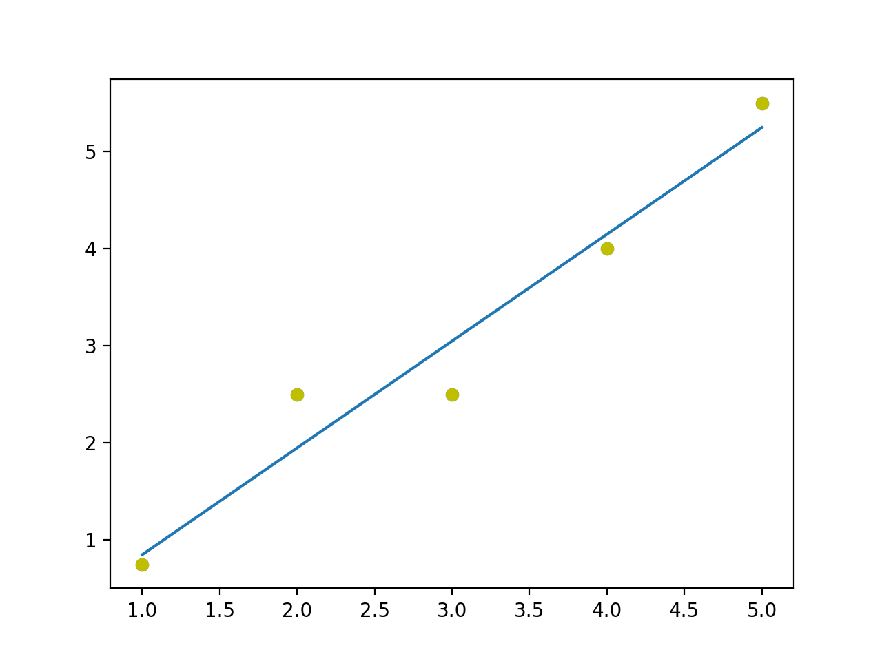
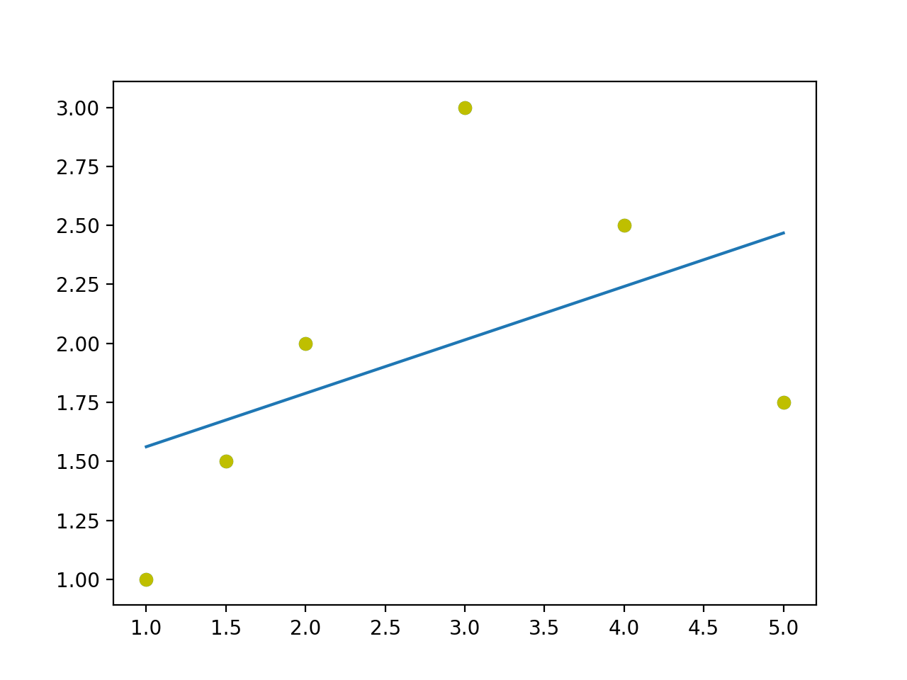
Functionally misspecifying our regression model will also introduce autocorrelation in our model. Consider the two plots shown below.
In the first plot the line fits the sample points properly. In the second one, it doesn’t fit properly. The sample points seem to form a curve of some sort while we try to fit a straight line through it. What we get is runs of negative residuals followed by positive residuals which indicates autocorrelation.
Autocorrelation can also be introduced not just by functionally misspecifying the regression model but also by the nature of data itself. For example, consider timeseries data representing stock market movement. The value of depends on i.e. the two are correlated.
When there is autocorrelation, the OLS estimators are no longer the best estimators for predicting the value of .
Conclusion
In this post we looked at the assumptions underlying OLS. In the coming post we’ll look at the Gauss-Markov theorem and the BLUE property of OLS estimators.
[1] There are also stochastic regression models where the values of X are not fixed.