In the previous post we looked at computing the Fibonacci series both with and without dynamic programming. In this post we’ll look at another example where dynamic programming is applicable. The example is borrowed from ‘Introduction to Algorithms’ by CLRS and implemented in Python. By the end of this post we’ll try to develop an intuition for when dynamic programming applies.

Rod Cutting

The problem we are presented with is the following: given a steel rod, we’d like to find the optimal way to cut it into smaller rods. More formally, we’re presented with a rod of size n inches and a table of prices p_i. We’d like to determine the maximum revenue r_n that we can obtain by cutting the rod and selling it. If the price p_n of the rod of length n is large enough, we may sell the rod without making any cuts.

The table of prices that we’ll work with is given below.

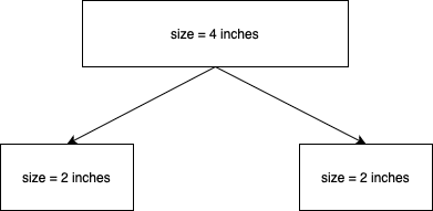
Consider a rod of length 4 inches. The maxium revenue we can obtain is 10 by cutting the rod into two parts of length 2 inches each.

Given a rod of n inches, we may sell it uncut or we may sell it by cutting it into smaller pieces. Since we do not know the size of the cuts to make, we will have to consider all possible sizes. Once we make a cut of size from the left end of the rod, we can view the remaining length of the rod of size as an independent instance of the rod cutting problem. In other words, we are solving a smaller instance of the same problem. The equation below shows how we can mathematically formulate the problem.

It states that the revenue r_n is the maximum revenue obtained by considering all cuts of size plus the revenue obtained by cutting the remaining rod of size . We can write a recursive function to obtain this value as follows:

1
2
3
4
5
6
7
8
9
10

def rod_cut(p: list[int], n: int) -> int:
    if n == 0:
        return 0

    q = float("-inf")

    for i in range(1, n + 1):
        q = max(q, p[i] + rod_cut(p, n - i))

    return q

We can verify the results by calling the function for a rod of size 4 and passing the table of prices.

1
2

p = [0, 1, 5, 8, 9, 10, 17, 17, 20, 24, 30]
assert 10 == rod_cut(p=p, n=4)

The recursive version, however, does redundant work. Consider the rod of size n = 4. We will have to consider cuts of size . When considering the remaining rod of size 3, we’d consider cuts of size . In both of these cases we recompute, for example, the revenue obtained when the remainder of the rod is of size 2.

We can use dynamic programming to solve this problem by modifying the rod_cut function as follows.

1
2
3
4
5
6
7
8
9
10
11
12
13
14
15

def rod_cut(p: list[int], t: list[int | None], n: int) -> int:
    if n == 0:
        return 0

    if t[n] is not None:
        return t[n]

    q = float("-inf")

    for i in range(1, n + 1):
        q = max(q, p[i] + rod_cut(p, t, n - i))

    t[n] = q

    return q

Notice how we’ve introduced a table t which stores the maximum revenue obtained by cutting a rod of size n. This allows us to reuse previous computations. We can run this function and verify the result.

1
2
3

t = [None] * 11
p = [0, 1, 5, 8, 9, 10, 17, 17, 20, 24, 30]
assert 10 == rod_cut(p, t, 4)

The question that we’re left with is the following: how did we decide that the problem could be solved with dynamic programming? There are two key factors that help us in deciding if dynamic programming can be used. The first is overlapping subproblems and the second is optimal substructure.

For a dynamic programming algorithm to work, the number of subproblems must be small. This means that the recursive algorithm which solves the problem encounters the same subproblems over and over again. When this happens, we say that the problem we’re trying to solve has overlapping subproblems. In the rod cutting problem, when we try to cut a rod of size 4, we consider cuts of size . When we, then, consider the remaining rod of size 3, we consider cuts of size . The smaller problem of optimally cutting the rod of size 2 is encountered again. In other words, it is an overlapping subproblem. Dynamic programming algorithms solve an overlapping subproblem once and store its result in a table so that it can be reused again.

The second factor is optimal substructure. When a problem exhibits optimal substructure, it means that the solution to the problem contains within it the optimal solutions to the subproblems; we build an optimal solution to the problem from optimal solutions to the subproblems. The rod-cutting problem exhibits optimal substructure because the optimal solution to cutting a rod of length involves finding the optimal solution to cutting the remaining rod, if a cut has been made.

Moving on. So far our algorithm has returned the optimal value of the solution. In other words, it returned the maximum revenue that can be obtained by optimaly cutting the rod. We often need to store the choice that led to the optimal solution. In the context of the rod cutting problem, this would be the lengths of the cuts made. We can do this by keeping additional information in a separate table. The following code listing is a modification of the above function with an additional table s to store the value of the optimal cut.

1
2
3
4
5
6
7
8
9
10
11
12
13
14
15
16
17
18
19
20
21

def rod_cut(p: list[int], s: list[int | None], t: list[int | None], n: int) -> int:
    if n == 0:
        return 0

    if t[n] is not None:
        return t[n]

    q = float("-inf")
    j = None

    for i in range(1, n + 1):
        r = p[i] + rod_cut(p, s, t, n - i)

        if r > q:
            q = r
            j = i

    s[n] = j
    t[n] = q

    return q

In this version of the code, we store the size of the cut being made for a rod of length n in the table s. Once we have this information, we can reconstruct the optimal solution. The function that follows shows how to do that.

1
2
3
4
5
6
7
8
9

def optimal_cuts(s: list[int | None], n: int) -> list[int]:
    cuts = []

    while n:
        cut = s[n]
        n = n - s[n]
        cuts.append(cut)

    return cuts

Finally, we call the function to see the optimal solution. Since we know that the optimal solution for a rod of size 4 is to cut it into two equal halves, we’ll use .

1
2
3
4
5
6
7

n = 4
t = [None] * 11
s = [None] * 11
p = [0, 1, 5, 8, 9, 10, 17, 17, 20, 24, 30]
q = rod_cut(p, s, t, n)

assert [2, 2] == optimal_cuts(s, n)

That’s it. That’s how we can use dynamic programming to optimally cut a rod of size inches.

In this post, and hopefully in the next few posts, I’d like to devle into the topic of dynamic programming. The aim is to develop an intuition for when it is applicable by solving a few puzzles. I’ll be referring to the chapter on dynamic programming in ‘Introduction to Algorithms’ by CLRS, and elucidating it in my own words.

Dynamic Programming

The chapter opens with the definition of dynamic programming: it is a technique for solving problems by combining solutions to subproblems. The subproblems may have subsubproblems that are common between them. A dynamic programming algorithm solves these subsubproblems only once and saves the result, thereby avoiding unnecessary work. The term “programming” refers to a tabular method in which the results of subsubproblems are saved in a table and reused when the same subsubproblem is encountered again.

All of this is abstract so let’s look at a concrete example of computing the Fibonacci series.

1
2

def fibonacci(n: int) -> int:
    return n if n < 2 else fibonacci(n - 1) + fibonacci(n - 2)

The call graph for fibonacci(4) is given below.

As we can see, we’re computing fibonacci(2) twice. In other words, the subsubproblem of computing fibonacci(2) is shared between fibonacci(4) and fibonacci(3). A dynamic programming algorithm would solve this subsubproblem only once and save the result in a table and reuse it. Let’s see what that looks like.

1
2
3
4
5
6
7
8
9

def fibonacci(n: int) -> int:
    T = [0, 1] + ([None] * (n - 2))
    return fibonacci_helper(n=n - 1, T=T)


def fibonacci_helper(n: int, T: list[int | None]) -> int:
    if T[n] is None:
        T[n] = fibonacci_helper(n - 1, T) + fibonacci_helper(n - 2, T)
    return T[n]

In the code above, we create a table T which stores the Fibonacci numbers. If an entry exists in the table, we return it immediately. Otherwise, we compute and store it. This recursive approach, with results of subsubproblems stored in a table, is called “top-down with memoziation”; the table is called the “memo”. We begin with the original problem and then proceed to solve it by finding solutions to smaller subproblems. The procedure which computes the solution is said to be “memoized” as it remembers the previous computations.

Another approach is called “bottom-up” in which the solutions to the smaller subproblems are computed first. This depends on the notion that subproblems have “size”. In this approach, a solution to the subproblem is found only when the solutions to its smaller subsubproblems have been found. We can apply this approach when computing the Fibonacci series.

1
2
3
4
5
6
7

def fibonacci(n: int) -> int:
    T = [0, 1] + ([None] * (n - 2))

    for i in range(2, n):
        T[i] = T[i - 1] + T[i - 2]

    return T[n - 1]

As we can see, the larger numbers in the Fibonacci series are computed only when the smaller numbers have been computed.

This was a small example of how dynamic programming algorithms work. They are applied to problems where subproblems share subsubproblems. The solutions to these subsubproblems are stored in a table and reused when they are encountered again. This enables the algorithm to work more efficiently as it avoids the rework of solving the subsubproblems.

In the next post we’ll look at another example of dynamic programming that’s presented in the book and implement it in Python to further our understanding of the subject.

I’d recently written about an experimental library to detect PII. When discussing it with an acquaintance of mine, I was told that PII can also be disguised. For example, a corpus of text like a review or a comment can contain email address in the form “johndoeatgmaildotcom”. This led me to update the library so that emails like these can also be flagged. In a nutshell, I had to update the regex which was used to find the email.

Example

This is best explained with a few examples. In all of the examples, we begin with a proper email and disguise it one step at a time.

1
2
3
4
5
6
7
8
9

column = Column(name="comment")
detector = ColumnValueRegexDetector()

assert detector.detect(column=column, sample="john.doe@provider.com") == Email()
assert detector.detect(column=column, sample="johndotdoe@provider.com") == Email()
assert detector.detect(column=column, sample="johndotdoeatproviderdotcom") == Email()
assert detector.detect(column=column, sample="john.doe@provider.co.uk") == Email()
assert detector.detect(column=column, sample="johndotdoeatproviderdotcodotuk") == Email()
assert detector.detect(column=column, sample="myemailis:john.doeatproviderdotcom") == Email()

All of these assertions pass and the regex detector is able to flag all of these examples as email.

I recently created an experimental library, detectpii, to detect PII data in relational databases. In this post we’ll take a look at the rationale behind the library and it’s architecture.

Rationale

A common requirement in many software systems is to store PII information. For example, a food ordering system may store the user’s name, address, phone number, and email. This information may also be replicated into the data warehouse. As a matter of good data governance, you may want to restrict access to such information. Many data warehouses allow applying a masking policy that makes it easier to redact such values. However, you’d have to specify which columns to apply this policy to. detectpii makes it easier to identify such tables and columns.

My journey into creating this library began by looking for open-source projects that would help identify such information. After some research, I did find a few projects that do this. The first project is piicatcher. It allows comparing the column names of tables against regular expressions that represent common PII column names like user_name. The second project is CommonRegex which allows comparing column values against regular expression patterns like emails, IP addresses, etc.

detectpii combines these two libraries to allow finding column names and values that may potentially contain PII. Out of the box, the library allows scanning column names and a subset of its values for potentially PII information.

Architecure

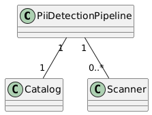
At the heart of the library is the PiiDetectionPipeline. A pipeline consists of a Catalog, which represents the database we’d like to scan, and a number of Scanners, which perform the actual scan. The library ships with two scanners - the MetadataScanner and the DataScanner. The first compares column names of the tables in the catalog against known patterns for the ones which store PII information. The second compares the value of each column of the table by retrieving a subset of the rows and comparing them against patterns for PII. The result of the scan is a list of column names that may potentially be PII.

The design of the library is extensible and more scanners can be added. For example, a scanner to use a proprietary machine learning algorithm instead of regular expression match.

Usage

To perform a scan, we create a pipeline and pass it a catalog and a list of scanners. To inititate the scan, we call the scan method on the pipeline to get back a list of PII columns.

1
2
3
4
5
6
7
8
9
10
11
12
13
14
15
16
17
18
19
20
21
22
23
24
25

from detectpii.catalog import PostgresCatalog
from detectpii.pipeline import PiiDetectionPipeline
from detectpii.scanner import DataScanner, MetadataScanner

# -- Create a catalog to connect to a database / warehouse
pg_catalog = PostgresCatalog(
    host="localhost",
    user="postgres",
    password="my-secret-pw",
    database="postgres",
    port=5432,
    schema="public"
)

# -- Create a pipeline to detect PII in the tables
pipeline = PiiDetectionPipeline(
    catalog=pg_catalog,
    scanners=[
        MetadataScanner(),
        DataScanner(percentage=20, times=2,),
    ]
)

# -- Scan for PII columns.
pii_columns = pipeline.scan()

That’s it. That’s how to use the library to detect PII columns in tables.

In the exercises that follow the chapter on algebraic manipulations, there is a question that pertains to expressing an integer as the sum of two other integers squared. We are then asked to find expressions for the multiples of , namely and . In this post, we’ll take a look at the solution provided by the authors for the first half of the question, , and then come up with a method of our own to solve the second half, .

Question

If is an integer that can be expressed as the sum of two integer squares, show that both and can also be expressed as the sum of two integer squares.

Solution

From the question, since it is the sum of two integer squares. This means . We need to find two integers such that when their squares are summed, we end with . From the solution, these are the numbers (a + b) and (a - b) because when they are squared and summed, we get . This is the result of . Go ahead and expand them to verify the result.

What do we deduce from this? We find that both the expressions contributed an and a . These were added together to get the final result. How do we use this to get ? Notice that we’re squaring the integers. This means that, for example, one of them would have to contribute an and the other would have to contribute a ; similar logic applies for .

This leaves us with two pairs of numbers — and . Let’s square and sum both of these numbers one-by-one.

What integers would we need for ?

In a previous post we’d seen how to create a realtime data platform with Pinot, Trino, Airflow, and Debezium. In this post we’ll see how to setup a data catalog using DataHub. A data catalog, as the name suggests, is an inventory of the data within the organization. Data catalogs make it easy to find the data within the organisation like tables, data sets, reports, etc.

Before we begin

My setup consists of Docker containers required to run DataHub. While DataHub provides features like data lineage, column assertions, and much more, we will look at three of the simpler featuers. One, we’ll look at creating a glossary of the terms that will be used frequently in the organization. Two, we’ll catalog the datasets and views that we saw in the previous post. Three, we’ll create an inventory of dashboards and reports created for various departments within the organisation.

The rationale for this as follows. Imagine a day in the life of a business analyst. Their responsibilities include creating reports and dashboards for various departments. For example, the marketing team may want to see an “orders by day” dashboard so that they can correlate the effects of advertising campaigns with an uptick in the volume of orders. Similarly, the product team may want a report of which features are being used by the users. The requests of both of these teams will be served by the business analyts using the data that’s been brought into the data platform. While they create these reports and dashboards, it’s common for them to receive queries asking where a team member can find a certain report or how to interpret a data point within a report. They may also have to search for tables and data sets to create new reports, acquaint themselves with the vocabulary of the various departments, and so on.

A data catalog makes all of this a more efficient process. In the following sections we’ll see how we can use DataHub to do it. For example, we’ll create the definition of the term “order”, create a list of reports created for the marketing department, and bring in the views and data sets so that they become searchable.

The work of data scientists is similar, too, because they create data sets that can be reused across various models. For example, data sets representing features for various customers can be stored in the platform, made searchable, and used with various models. They, too, benefit from having a data catalog.

Finally, it helps bring people up to speed with the data that is consumed by their department or team. For example, when someone joins the marketing team, pointing them to the data catalog helps them get productive quickly by finding the relevant reports, terminology, etc.

Ingesting data sets and views

To ingest the tables and views, we’ll create a data pipeline which ingets metadata from AWS Glue and writes it to the metadata service. This is done by creating a YAML configuration in DataHub that specifies where to ingest the metadata from, and where to write it. Once this is created, we can schedule it to run periodically so that it stays updated with Glue.

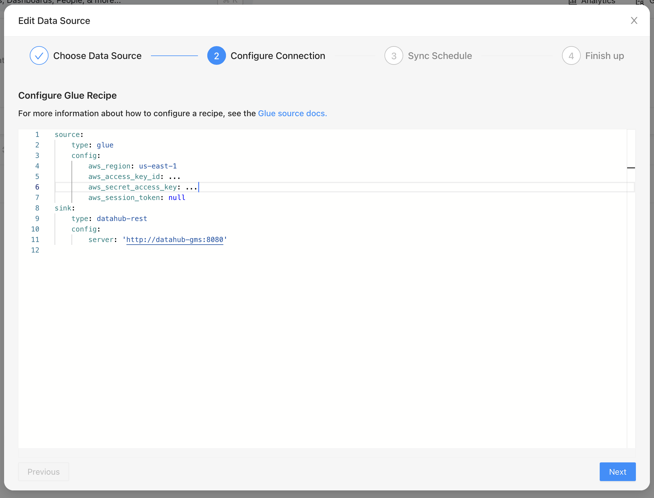
The image above shows how we define a “source” and how we ingest it into a “sink”. Here we’ve specified that we’d like to read from Glue and write it to DataHub’s metadata service.

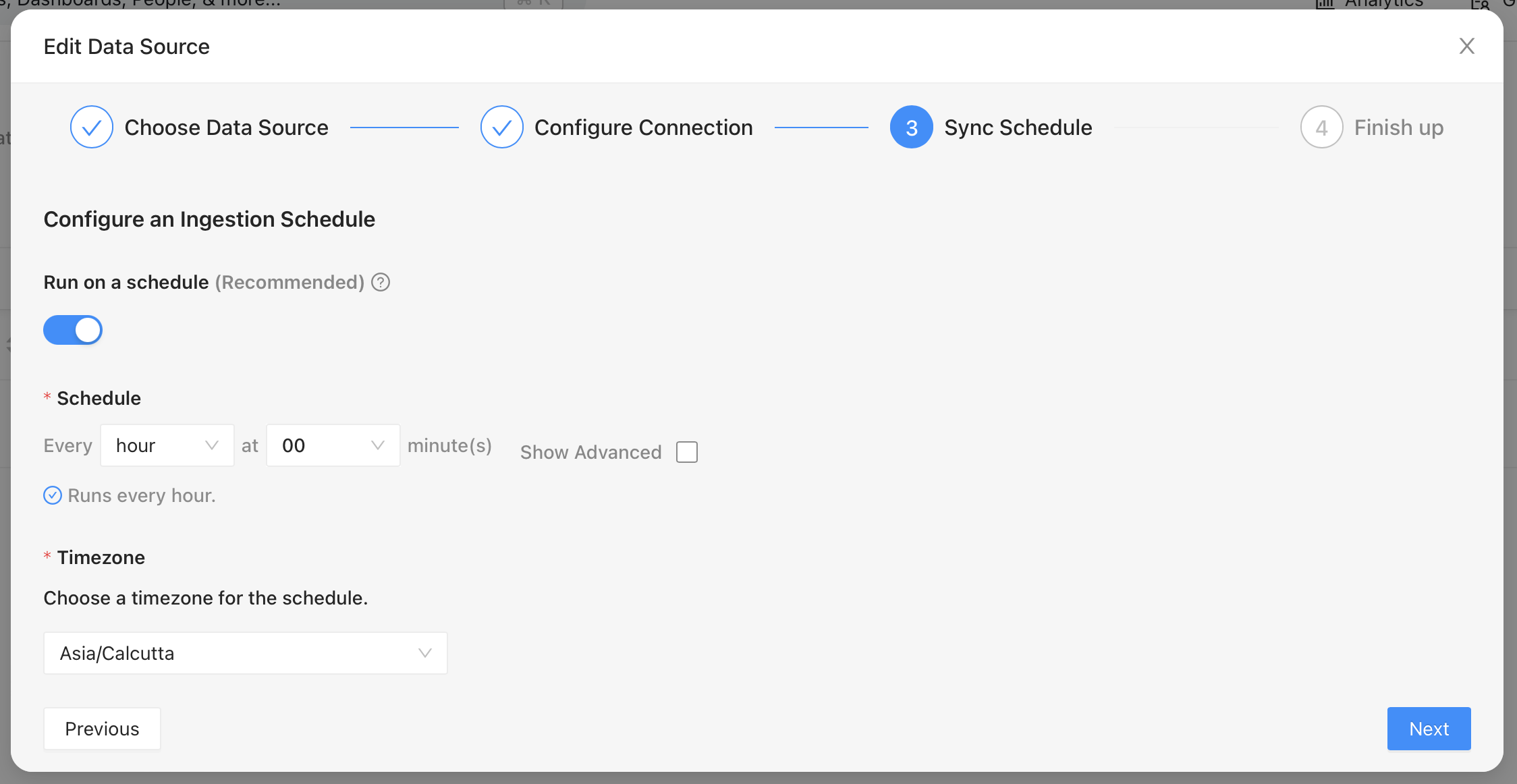
Once the source and destination are defined, we can set a schedule to run the ingestion. This will bring in the metadata about the data sets and views we’ve created in Glue.

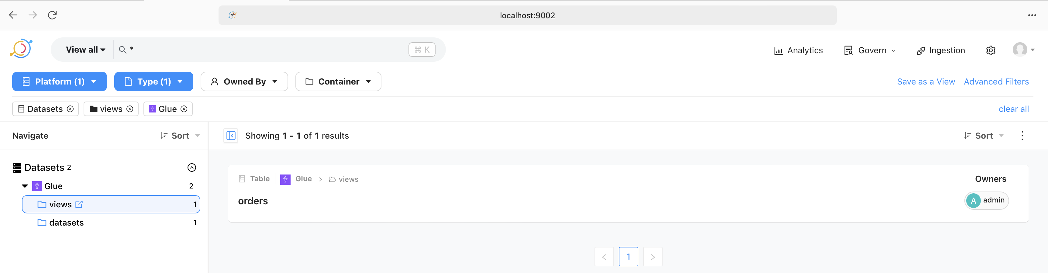
The image above shows that a successful run of the ingestion pipeline brings in the views and data sets. These are then browsable in the UI. Similarly, they are also searchable as shown in the following image.

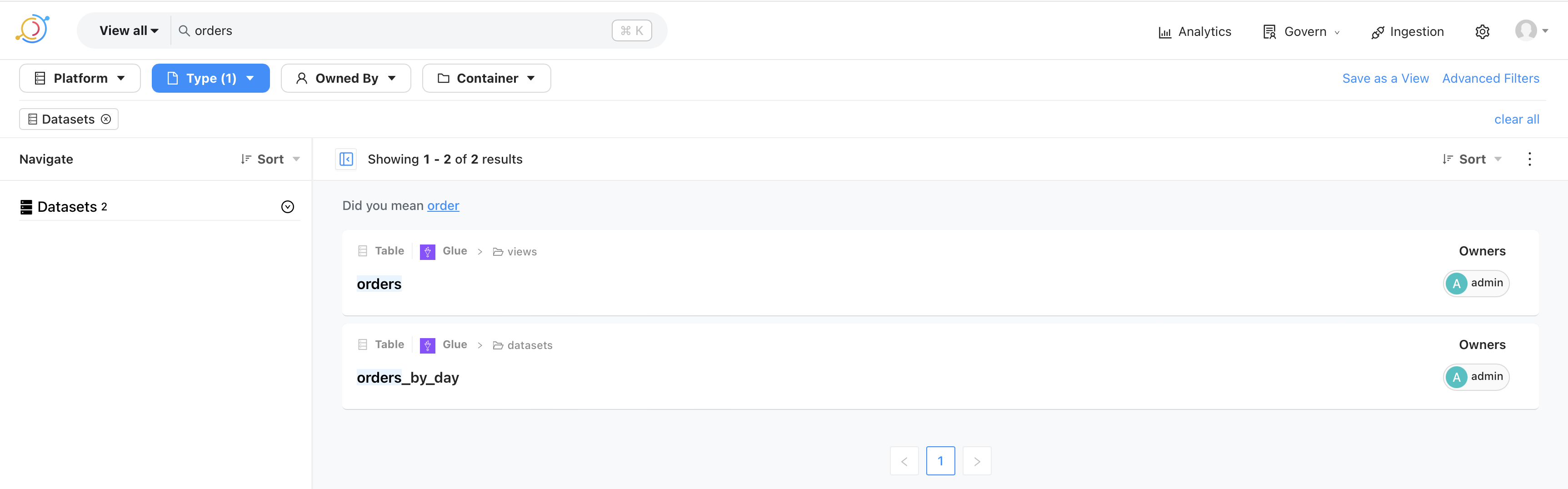
This makes it possible for the analysts and the data scientists to quickly locate data sets.

Defining the vocabulary

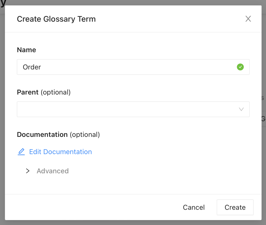
Next, we’ll create the definition of the word “order”. This can be done from the UI as shown below. The definition can be added by editing the documentation.

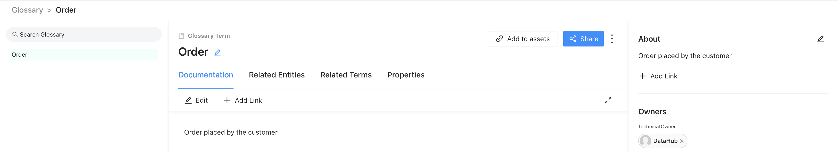
Once created, this is available under “Glossary” and in search results.

Data products

Finally, we’ll create a data product. This is the catalog of reports and dashboards created for various departments. For example, the image below shows a dashboard created for the marketing team.

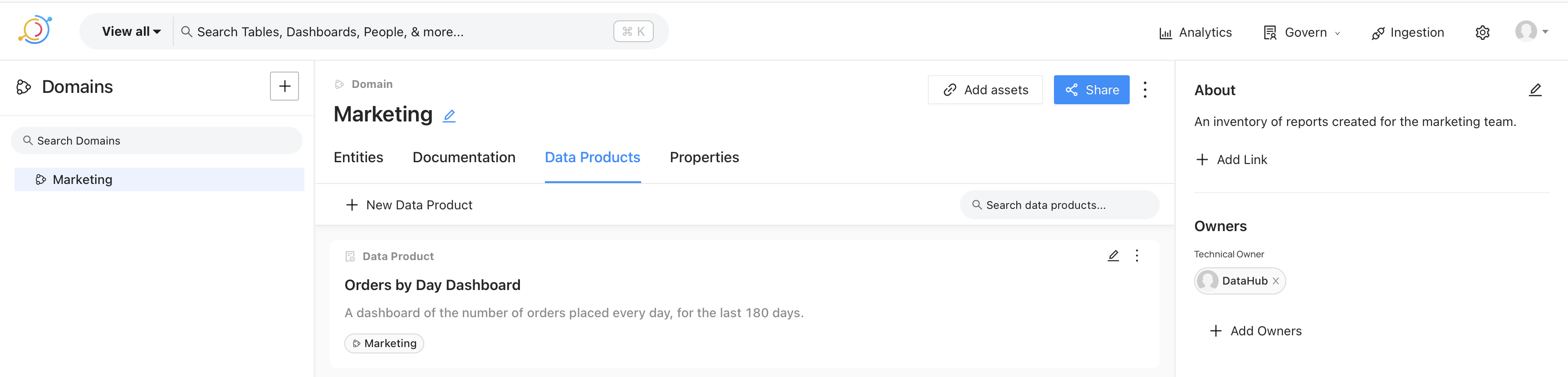
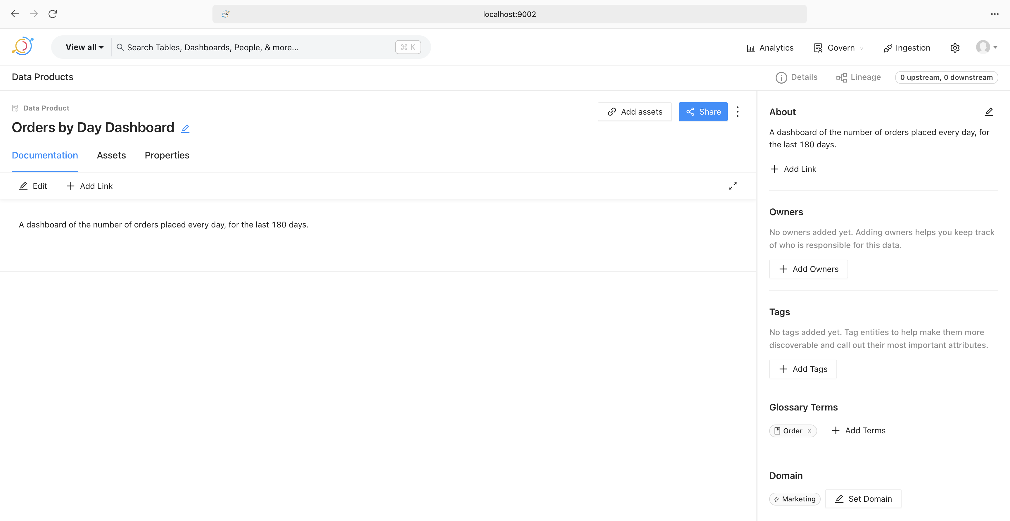
Expanding the dashboard allows us to look at the documentation for the report. This could contain the definition of the terms used in the report, as shown on the bottom right, a link to the dashboard in Superset, definitions of data points, report owners, and so on.

That’s it. That’s how a data catalog helps streamline working with data.

As I continue working my way through the book on programming puzzles, I came across those involving permutations. In this post I’ll collect puzzles with the same theme, both from the book and from the internet.

All permutations

The first puzzle is to compute all the permutations of a given array. By extension, it can be used to compute all the permutations of a string, too, if we view it as an array of characters. To do this we’ll implement Heap’s algorithm. The following is its recursive version.

1
2
3
4
5
6
7
8
9
10
11
12
13

def heap(permutations: list[list], A: list, n: int):
    if n == 1:
        permutations.append(list(A))
    else:
        heap(permutations, A, n - 1)

        for i in range(n - 1):
            if n % 2 == 0:
                A[i], A[n - 1] = A[n - 1], A[i]
            else:
                A[0], A[n - 1] = A[n - 1], A[0]

            heap(permutations, A, n - 1)

The array permutations is the accumulator which will store all the permutations of the array. The initial arguments to the function would be an empty acuumulator, the list to permute, and the length of the list.

Next permutation

The next puzzle we’ll look at is computing the next permutation of the array in lexicographical order. The following implementation has been taken from the book.

1
2
3
4
5
6
7
8
9
10
11
12
13
14
15
16
17

def next_permutation(perm: list[int]) -> list[int]:
    inversion_point = len(perm) - 2

    while (inversion_point >= 0) and (perm[inversion_point] >= perm[inversion_point + 1]):
        inversion_point = inversion_point - 1

    if inversion_point == -1:
        return []

    for i in reversed(range(inversion_point + 1, len(perm))):
        if perm[i] > perm[inversion_point]:
            perm[inversion_point], perm[i] = perm[i], perm[inversion_point]
            break

    perm[inversion_point + 1:] = reversed(perm[inversion_point + 1:])

    return perm

Previous permutation

A variation of the puzzle is to compute the previous permutation of the array in lexicographical order. The idea is to “reverse” the logic for computing the next permutation. If we look closely, we’ll find that all we’re changing are the comparison operators.

1
2
3
4
5
6
7
8
9
10
11
12
13
14
15
16
17

def previous_permutation(perm: list[int]) -> list[int]:
    inversion_point = len(perm) - 2

    while (inversion_point >= 0) and (perm[inversion_point] <= perm[inversion_point + 1]):
        inversion_point = inversion_point - 1

    if inversion_point == -1:
        return []

    for i in reversed(range(inversion_point + 1, len(perm))):
        if perm[i] < perm[inversion_point]:
            perm[inversion_point], perm[i] = perm[i], perm[inversion_point]
            break

    perm[inversion_point + 1:] = reversed(perm[inversion_point + 1:])

    return perm

kth smallest permutation

The final puzzle we’ll look at is the one where we need to compute the k’th smallest permutation. The solution to this uses the previous_permutation function that we saw above. The idea is to call this function k times on the lexicographically-largest array. Sorting the array in decreasing order results is the largest. This becomes the input to the previous_permutation function.

1
2
3
4
5
6
7
8
9

def kth_smallest_permutation(perm: list[int], k: int) -> list[int]:
    # -- Arrange the numbers in decreasing order
    # -- thereby creating the lexicographically largest permutation
    perm = sorted(perm, reverse=True)

    for _ in range(k):
        perm = previous_permutation(perm)

    return perm

That’s it. These are puzzles involving permutations.

I am working my way through a classic book of programming puzzles. As I work through more of these puzzles, I’ll share what I discover to solidify my understanding and help others who are doing the same. If you’ve ever completed puzzles on a site like leetcode, you’ll notice that the sheer volume of puzzles is overwhelming. However, there are patterns to these puzzles, and becoming familiar with them makes it easier to solve them. In this post we’ll take a look at one such pattern - two pointers - and see how it can be used to solve puzzles involving arrays.

Two Pointers

The idea behind two pointers is that there are, as the name suggests, two pointers that traverse the array, with one pointer leading the other. Using these two pointers we update the array and solve the puzzle at hand. As an illustrative example, let us consider the puzzle where we’re given an array of even and odd numbers and we’d like to move all the even numbers to the front of the array.

Even and Odd

1
2
3
4
5
6
7
8
9
10
11

def even_odd(A: list[int]) -> None:
    """Move even numbers to the front of the array."""
    write_idx = 0
    idx = 0

    while idx < len(A):
        if A[idx] % 2 == 0:
            A[write_idx], A[idx] = A[idx], A[write_idx]
            write_idx = write_idx + 1

        idx = idx + 1

The two pointers here are idx and write_idx. While idx traverses the array and indicates the current element, write_idx indicates the position where the next even number should be written. Whenever idx points to an even number, it is written at the position indicated by write_idx. With this logic, if all the numbers in the array are even, idx and write_idx point to the same element i.e. the number is swapped with itself and the pointers are moved forward.

We’ll build upon this technique to remove duplicates from the array.

Remove Duplicates

Consider a sorted array containing duplicate numbers. We’d like to keep only one occurrence of each number and overwrite the rest. This can be solved using two pointers as follows.

1
2
3
4
5
6
7
8
9
10
11
12

def remove_duplicates(A: list[int]) -> int:
    """Remove all duplicates in the array."""
    write_idx, idx = 1, 1

    while idx < len(A):
        if A[write_idx - 1] != A[idx]:
            A[write_idx] = A[idx]
            write_idx = write_idx + 1

        idx = idx + 1

    return write_idx

In this solution, idx and write_idx start at index 1 instead of 0. The reason is that we’d like to look at the number to the left of write_idx, and starting at index 1 allows us to do that. Notice also how we’re writing the if condition to check for duplicity in the vicinity of write_idx; the number to the left of write_idx should be different from the one that idx is presently pointing to.

As a varitation, move the duplicates to the end of the array instead of overwriting them.

1
2
3
4
5
6
7
8
9
10
11
12

def remove_duplicates(A: list[int]) -> None:
    """Remove all duplicates in the array and move them to the end"""
    write_idx, idx = 1, 1

    while idx < len(A):
        if A[write_idx - 1] != A[idx]:
            A[write_idx], A[idx] = A[idx], A[write_idx]
            write_idx = write_idx + 1

        idx = idx + 1

    return write_idx

As another variation, remove a given number from the array by moving it to the end.

1
2
3
4
5
6
7
8
9
10

def remove(A: list[int], k: int) -> None:
    write_idx = 0
    idx = 0

    while idx < len(A):
        if A[idx] != k:
            A[write_idx], A[idx] = A[idx], A[write_idx]
            write_idx = write_idx + 1

        idx = idx + 1

With this same pattern, we can now change the puzzle to state that we want at most two instances of the number in the sorted array.

Remove Duplicates Variation

1
2
3
4
5
6
7
8
9
10

def remove_duplicates(A: list[int]) -> int:
    """Keep at most two instances of the number."""
    write_idx = 2

    for idx in range(2, len(A)):
        if A[write_idx - 2] != A[idx]:
            A[write_idx] = A[idx]
            write_idx = write_idx + 1

    return write_idx

Akin to the previous puzzle, we look for duplicates in the vicinity of write_idx. While in the previous puzzle the if condition checked for one number to the left, in this variation we look at two positions to the left of write_idx to keep at most two instances. The remainder of the logic is the same. As a variation, try keeping at most three instances of the number in the sorted array.

Finally, we’ll use the same pattern to solve the Dutch national flag problem.

Dutch National Flag

In this problem, we sort the array by dividing it into three distinct regions. The first region contains elements less than the pivot, the second region contains elements equal to the pivot, and the third region contains elements greater than the pivot.

1
2
3
4
5
6
7
8
9
10
11
12
13
14
15
16
17
18
19
20
21
22
23

def dutch_national_flag(A: list[int], pivot_idx: int) -> None:
    """Divide the array into three distinct regions."""
    pivot = A[pivot_idx]
    write_idx = 0
    idx = 0

    # --- Move all elements less than pivot to the front
    while idx < len(A):
        if A[idx] < pivot:
            A[write_idx], A[idx] = A[idx], A[write_idx]
            write_idx = write_idx + 1
        idx = idx + 1

    idx = write_idx

    # -- Move all elements equal to the pivot to the middle
    while idx < len(A):
        if A[idx] == pivot:
            A[write_idx], A[idx] = A[idx], A[write_idx]
            write_idx = write_idx + 1
        idx = idx + 1

    # -- All elements greater than pivot have been moved to the end.

This problem combines everything we’ve seen so far about two pointers and divides the array into three distinct regions. As we compute the first two regions, the third region is computed as a side-effect.

We can now solve a variation of the Dutch national flag partitioning problem by accepting a list of pivot elements. In this variation all the numbers within the list of pivots appear together i.e. all the elements equal to the first pivot element appear first, equal to second pivot element appear second, and so on.

1
2
3
4
5
6
7
8
9
10
11
12

def dutch_national_flag(A: list[int], pivots: list[int]) -> None:
    """This is a variation in which all elements with same key appear together."""
    write_idx = 0

    for pivot in pivots:
        idx = write_idx

        while idx < len(A):
            if A[idx] == pivot:
                A[write_idx], A[idx] = A[idx], A[write_idx]
                write_idx = write_idx + 1
            idx = idx + 1

That’s it, that’s how we can solve puzzles involving two pointers and arrays.

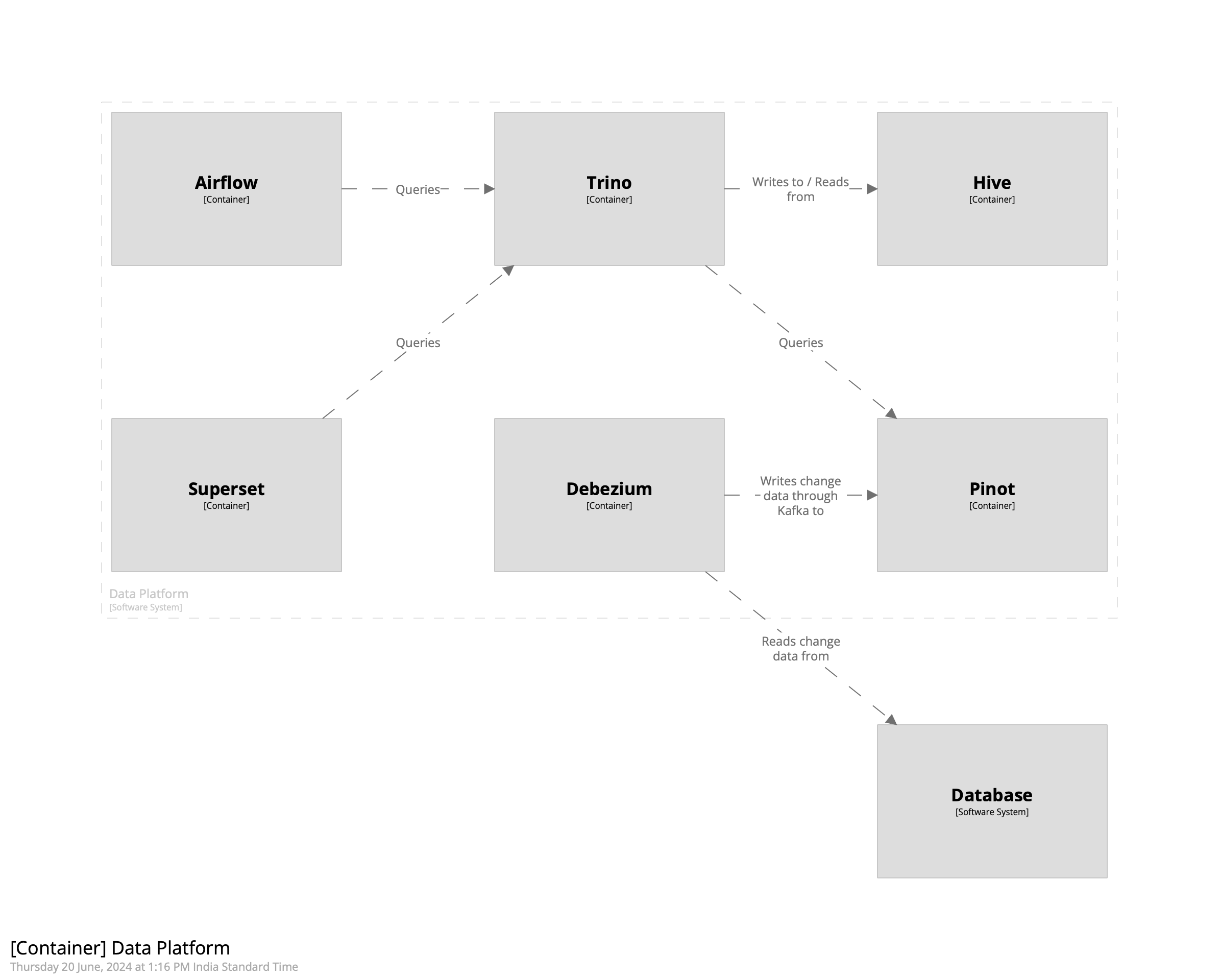
I’d previously written about creating a realtime data warehouse with Apache Doris and Debezium. In this post we’ll see how to create a realtime data platform with Pinot, Trino, Airflow, Debezium, and Superset. In a nutshell, the idea is to bring together data from various sources into Pinot using Debezium, transform it using Airflow, use Trino for query federation, and use Superset to create reports.

Before We Begin

My setup consists of Docker containers for running Pinot, Airflow, Debezium, and Trino. Like in the post on creating a warehouse with Doris, we’ll create a person table in Postgres and replicate it into Kafka. We’ll then ingest it into Pinot using its integrated Kafka consumer. Once that’s done, we’ll use Airflow to transform the data to create a view that makes it easier to work with it. Finally, we can use Superset to create reports. The intent of this post is to create a complete data platform that makes it possible to derive insights from data with minimal latency. The overall architecture looks like the following.

Getting Started

We’ll begin by creating a schema for the person table in Pinot. This will then be used to create a realtime table. Since we want to use Pinot’s upsert capability to maintain the latest record of each row, we’ll ensure that we define the primary key correctly in the schema. In the case of the person table, it is the combination of the id and the customer_id field. The schema looks as follows.

1
2
3
4
5
6
7
8
9
10
11
12
13
14
15
16
17
18
19
20
21
22
23
24
25
26
27
28
29
30
31
32
33

{
    "schemaName": "person",
    "dimensionFieldSpecs": [
        {
            "name": "id",
            "dataType": "LONG"

        },
        {
            "name": "customer_id",
            "dataType": "LONG"
        },
        {
            "name": "source",
            "dataType": "JSON"
        },
        {
            "name": "op",
            "dataType": "STRING"
        }
    ] ,
    "dateTimeFieldSpecs": [{
        "name": "ts_ms",
        "dataType": "LONG",
        "format" : "1:MILLISECONDS:EPOCH",
        "granularity": "1:MILLISECONDS"
    }],
    "primaryKeyColumns": [
        "id",
        "customer_id"
    ],
    "metricFieldSpecs": []
}

We’ll use the schema to create the realtime table in Pinot. Using ingestionConfig we’ll extract fields out of the Debezium payload and into the columns defined above. This is defined below.

1
2
3
4
5
6
7
8
9
10
11
12
13
14
15
16
17
18
19
20

"ingestionConfig":{
      "transformConfigs":[
        {
            "columnName": "id",
            "transformFunction": "jsonPath(payload, '$.after.id')"
        },
        {
            "columnName": "customer_id",
            "transformFunction": "jsonPath(payload, '$.after.customer_id')"
        },
        {
           "columnName": "source",
           "transformFunction": "jsonPath(payload, '$.after')"
        },
        {
          "columnName": "op",
          "transformFunction": "jsonPath(payload, '$.op')"
        }
      ]
   }

Next we’ll create a table in Postgres to store the entries. The SQL query is given below.

1
2
3
4
5
6

CREATE TABLE person (
    id BIGSERIAL NOT NULL,
    customer_id BIGINT NOT NULL,
    name TEXT NOT NULL,
    PRIMARY KEY (id, customer_id)
);

Next we’ll create a Debezium source connector to stream change data into Kafka.

1
2
3
4
5
6
7
8
9
10
11
12
13
14
15
16
17
18
19
20
21
22
23
24
25

{
    "name": "person",
    "config": {
        "connector.class": "io.debezium.connector.postgresql.PostgresConnector",
        "database.hostname": "db",
        "database.user": "postgres",
        "database.password": "my-secret-pw",
        "database.dbname": "postgres",
        "database.server.name": "postgres",
        "table.include.list": ".*\\.person",
        "plugin.name": "pgoutput",
        "publication.autocreate.mode": "filtered",
        "time.precision.mode": "connect",
        "tombstones.on.delete": "false",
        "snapshot.mode": "initial",
        "heartbeat.interval.ms": "1000",
        "transforms": "route",
        "transforms.route.type": "org.apache.kafka.connect.transforms.RegexRouter",
        "transforms.route.regex": "([^.]+)\\.([^.]+)\\.([^.]+)",
        "transforms.route.replacement": "$3",
        "event.processing.failure.handling.mode": "skip",
        "producer.override.compression.type": "snappy",
        "topic.prefix": "user_service"
    }
}

Finally, we’ll use curl to send these configs to their appropriate endpoints, beginning with Debezium.

1

curl -H "Content-Type: application/json" -XPOST -d @debezium/person.json localhost:8083/connectors | jq .

To create a table in Pinot we’ll first create the schema followed by the table. The curl command is given below.

1

curl -F schemaName=@tables/001-person/person_schema.json localhost:9000/schemas | jq .

The command to create the table is given below.

1

curl -XPOST -H 'Content-Type: application/json' -d @tables/001-person/person_table.json localhost:9000/tables | jq .

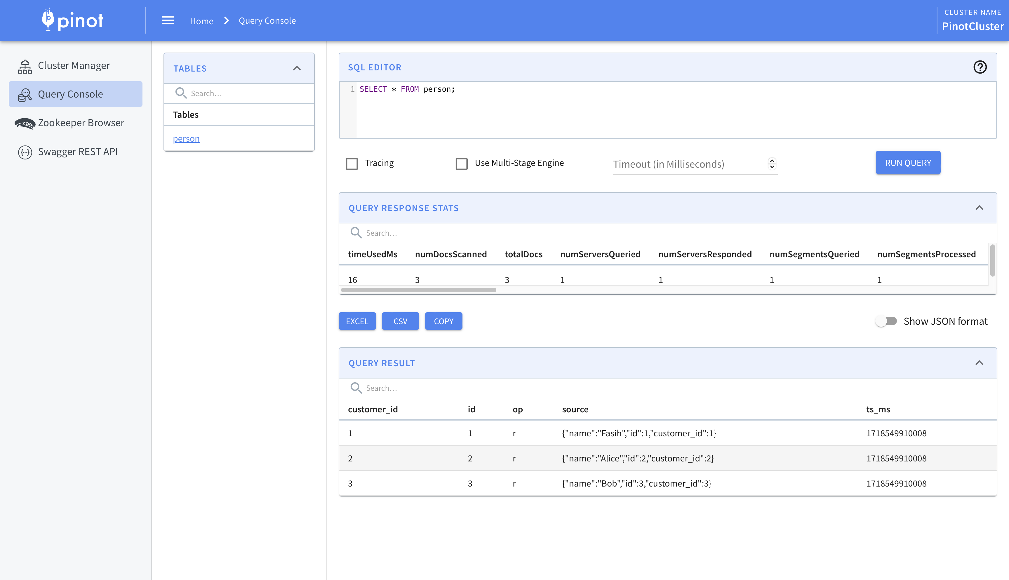
With these steps done, the change data from Debezium will be ingested into Pinot. We can view this using Pinot’s query console.

This is where we begin to integrate Airflow and Trino. While the data has been ingested into Pinot, we’ll use Trino for querying. There are two main reasons for this. One, this allows usto federate queries across multiple sources. Two, Pinot’s SQL capabilities are limited. For example, there is no support, as of writing, for creating views. To circumvent these we’ll create a Hive connector in Trino and use it to query Pinot.

The first step is to connect Trino and Pinot. We’ll do this using the Pinot connector.

1
2
3
4

CREATE CATALOG pinot USING pinot 
WITH (
    "pinot.controller-urls" = 'pinot-controller:9000'
);

Next we’ll create the Hive connector. This will allow us to create views, and more importantly materialized views which act as intermediate datasets or final reports, which can be queried by Superset. I’m using AWS Glue instead of Hive so you’ll have to change the configuration accordingly.

1
2
3
4
5
6
7
8
9
10
11
12

CREATE CATALOG hive USING hive
WITH (
    "hive.metastore" = 'glue',
    "hive.recursive-directories" = 'true',
    "hive.storage-format" = 'PARQUET',
    "hive.insert-existing-partitions-behavior" = 'APPEND',
    "fs.native-s3.enabled" = 'true',
    "s3.endpoint" = 'https://s3.us-east-1.amazonaws.com',
    "s3.region" = 'us-east-1',
    "s3.aws-access-key" = '...',
    "s3.aws-secret-key" = '...'
);

We’ll create a schema to store the views and point it to an S3 bucket.

1
2
3
4

CREATE SCHEMA hive.views
WITH (
    "location" = 's3://your-bucket-name-here/views/'
);

We can then create a view on top of the Pinot table using Hive.

1
2
3
4
5
6

CREATE OR REPLACE VIEW hive.views.person AS
SELECT id,
       customer_id,
       JSON_EXTRACT_SCALAR(source, '$.name') AS name,
       op
FROM pinot.default.person;

Finally, we’ll query the view.

1
2
3
4
5
6
7

trino> SELECT * FROM hive.views.person;
 id | customer_id | name  | op
----+-------------+-------+----
  1 |           1 | Fasih | r
  2 |           2 | Alice | r
  3 |           3 | Bob   | r
(3 rows)

While this helps us ingest and query the data, we’ll take this a step further and use Airflow to create the views instead. This allows us to create views which are time-constrained. For example, if we have an order table which contains all the orders placed by the customers, using Airflow allows to create views which are limited to, say, the last one year by adding a WHERE clause.

We’ll use the TrinoOperator that ships with Airflow and use it to create the view. To do this, we’ll create an sql folder under the dags folder and place our query there. We’ll then create the DAG and operator as follows.

1
2
3
4
5
6
7
8
9
10
11
12
13

dag = DAG(
    dag_id="create_views",
    catchup=False,
    schedule="@daily",
    start_date=pendulum.now("GMT")
)

person = TrinoOperator(
    task_id="person",
    trino_conn_id="trino",
    sql="sql/views/person.sql",
    dag=dag
)

Workflow

The kind of workflow this setup enables is the one where the data engineering team is responsible for ingesting the data into Pinot and creating the base views on top of it. The business intelligence / analytics engineering, and data science teams can then use Airflow to create datasets that they need. These can be created as materialized views to speed up reporting or training of machine learning models. Another advantage of this setup is that bringing in older data, say, of the last two years instead of one, is a matter of changing the query of the base view. This avoids complicated backfills and speeds things up significantly.

As an aside, it is possible to use DBT instead of TrinoOperator. It can be used in conjunction with TrinoOperator, too. However, I preferred using the in-built operator to keep the stack simpler.

Cost

Before we conclude, we’ll quickly go over how to keep the cost of the Pinot cluster low while using this setup. In the official documentation it says that data can be seperated by age; older data can be stored in HDDs while the newer data can be stored in SSDs. This allows lowering the cost of the cluster.

An alternative approach is to keep all the data in HDDs and load subsets into Hive for querying. This also allows changing the date range of the views by simply updating the queries. In essence, Pinot becomes the permanent storage for data while Trino and Hive become the intermediate query and storage layer.

That’s it. That’s how we can create a realtime data platform using Pinot, Trino, Debezium, and Airflow.

In the chapter on exponents the authors mention that if a base is raised to both a power and a root, we should calculate the root first and then the power. This works perfectly well. However, reversing the order produces correct results, too. In this post we’ll see why that works using the properties of exponents.

Let’s say we have a base that is raised to power and root . We could write this as . From the properties of exponents, we could rewrite this as . Alternatively, it can be written as . Since multiplication is commutative, we can switch the order of operations and rewrite it as . This means we can calculate the power first and then take the root.

Let’s take a look at a numerical example. Consider . We know that the answer should be equal to . If we were to calculate the root first, we get . If we were to calculate the power first and then take the root, we’d get . As we can see, we get the same result.

Therefore, we can apply the operations in any order.

While reading through the chapter on solving quadratics of a math textbook, I came across a paragraph where the authors mention that factoring quadratics takes a bit of ingenuity, experience, and dumb luck. I spent some time creating an alternative method from the one mentioned in the book which makes factoring quadratics a matter of following a simple set of steps, and removes the element of luck from it. In this post I will review some of the concepts mentioned in the book, and solve through one of the more difficult problems to illustrate my method.

Concepts

Let’s begin by looking at the quadratic . This can be factored as . Multiplying the terms gives us . Comparing this to the coefficients of the the original quadratic gives us , and . For a simple quadratic, we can guess that and . For quadratics where it is not so obvious, we need hints to guide us along the way.

We can get insights into the signs of and by looking at the product and the sum of coefficients of the quadratic. If the product is positive, then they have the same signs. If the product is negative, they have different signs. This makes intuitive sense. In case the product is positive, the sum tells us whether they are both positive or both negative.

We will use this again when we look at the alternative method to factor a quadratic. First, however, we will look at a different type of quadratic where the coefficient of is not 1.

Consider the quadratic . It can be factored as . Multiplying the terms gives us . As in the previously mentioned quadratic, we can get the product and the sum terms by comparing the quadratic with the general form we just derived. Here , and . A small nuance to keep in mind is that if the coefficient of were negative, we’d factor out a to make it positive.

Now we move on to the problem and the method. You’ll find that although the method is tedious, it will remove the element of luck from the process.

Method

Consider the quadratic . Here, , , and . From the guiding hints mentioned in the previous section, we notice that the signs of and are the same; they are either both positive or both negative. We begin the method be defining a function which returns a set of pairs of all the factors of . Therefore, we can write and as follows.

We will now get to the tedious part. We will create combinations of . We pick the first pair of factors of and match it with the first pair of factors of . For the sake of brevity, we will only some of the examples to illustrate the process.

Notice how we swap the values of and in the columns above. This is because we’re trying to find the product and its value will change depending on what the value of and are. Similarly, we’ll have to swap the values of and ; this is not apparent in the table above because both the values are . We will have to continue on with the table since we we are yet to find a combination of numbers which equals . The table is quite large so we’ll skip the rest of the entries for the sake of brevity and look at the one which gives us the value we’re looking for.

We can now write our factors as . This gives us or .

That’s it. That’s how we can factor quadratics by creating combinations of the factors of their coefficients.

In a previous blog post we’d seen how to use OpenTelemetry and Parca to instrument two microservcies. Imagine that our architecture has grown and we now have many microservices. For example, there is a microservice that is used to send emails, another which keeps track of user profile information, etc. We’d previously hardcoded the HTTP address of the second microservice to make a call from the first microservice. We could have, in a production environment, added a DNS entry which points to the load balancer and used that instead. However, when there are many microservcies, it becomes cumbersome to add these entries. Furthermore, any new microservice which depends on another microservice now needs to have the address as a part of its configuration. Maintaining a single repository, which can be used to find the microservices and their addresses, becomes difficult to maintain. An easier way to find services is to use service discovery - a dynamic way for one service to find another. In this post we’ll modify the previous architecture and add service discovery using Zookeeper.

Before We Begin

In a nutshell, we’ll use Zookeeper for service registration and discovery. We’ll modify our create_app factory function to make one more function call which registers the service as it starts. The function call creates an ephemeral node in Zookeeper at a specified path and stores the host and port. Any service which needs to find another service looks for it on the same path. We’ll create a small library for all of this which will make things easier.

Getting Started

We’ll begin by creating a simple attr class to represent a service.

1
2
3
4

@define(frozen=True)
class Service:
    host: str
    port: int

We’ll be using the kazoo Python library to interact with Zookeeper. The next step is to create a private variable which will be used to store the Zookeeper client.

1

_zk: KazooClient | None = None

Next we’ll add the function which will be called as a part of the create_app factory function.

1
2
3

def init_zookeeper_and_register():
    _init_zookeeper()
    _register_service()

In this function we’ll first initialize the connection to Zookeeper and then register our service. We’ll see both of these functions next, starting with the one to init Zookeeper.

1
2
3
4
5
6
7

def _init_zookeeper():
    global _zk

    if not _zk:
        _zk = KazooClient(hosts='127.0.0.1:2181')
        _zk.start(timeout=5)
        _zk.add_listener(_state_change_listener)

The _zk variable is meant to be a singleton. I was unable to find whether this is thread-safe or not but for the sake of this post we’ll assume it is. The start method creates a connection to Zookeeper synchronously and raises an error if no connection could be made in timeout seconds. We also add a listener to respond to changes in the state of a Zookeeper connection. This enables us to respond to scenarios where the connection drops momentarily. Since we’ll be creating ephemeral nodes in Zookeeper, they’ll be removed in the case of a session loss and would need to be recreated. In the listener we recreate the node upon a successful reconnection.

Next we’ll look at the function to register the service.

1
2
3
4
5
6
7
8
9
10
11
12
13
14
15
16
17

def _register_service():
    global _zk

    service = os.environ.get("SERVICE")
    host = socket.getfqdn()
    port = os.environ.get("PORT")

    assert service
    assert host
    assert port

    identifier = str(uuid4())
    path = f"/providers/{service}/{identifier}"
    data = {"host": host, "port": int(port)}
    data_bytes = json.dumps(data).encode("utf-8")

    _zk.create(path, data_bytes, ephemeral=True, makepath=True)

We get the name of the service and the port it is running on as environment variables. The host is retrieved as the fully-qualified domain name of the machine we’re on. Although the example is running on my local machine, it may work on a cloud provider like AWS. We then create a UUID identifier for the service, and a path on which the service will be registered. The information stored on the path is a JSON containing the host and the port of the service. Finally, we create an ephemeral node on the path and store the host and port.

Next we’ll look at the function which handles changes in connection state.

1
2
3

def _state_change_listener(state):
    if state == KazooState.CONNECTED:
        _register_service()

We simply re-register the service upon reconnection.

Finally, we’ll look at the function which retrieves an instance of the service from Zookeeper.

1
2
3
4
5
6
7
8
9
10
11
12
13
14
15
16
17
18

def get_service_from_zookeeper(service: str) -> Service | None:
    global _zk
    assert _zk

    path = f"/providers/{service}"
    children = _zk.get_children(path)

    if not children:
        return None

    idx = random.randint(0, len(children) - 1)

    child = children[idx]
    config, _ = _zk.get(f"/providers/{service}/{child}")
    config = config.decode("utf-8")
    config = json.loads(config)

    return Service(**config)

To get a service we get all the children at the path /providers/SERVICE_NAME. This returns a list of UUIDs, each of which represents an instance of the service. We randomly pick one of these instances and fetch the information associated with it. What we get back is a two-tuple containing the host and port, and an instance of ZStat which we can ignore. We decode and parse the returned information to get an instance of dict. This is then used to return an instance of Service. We can then use this information to make a call to the returned service.

This is all we need to create a small set of utility functions to register and discover services. All we need to do to register the service as a part of the Flask application process is to add a function call in the create_app factory function.

1
2
3
4
5
6
7
8

def create_app() -> Flask:
    ...

    # -- Initialize Zookeeper and register the service.
    init_zookeeper_and_register()

    return app

Finally, we’ll retrieve the information about the second service in the first service right before we make the call.

1
2
3
4

def make_request() -> dict:
    service = get_service_from_zookeeper(service="second")
    url = f"http://{service.host}:{service.port}"
    ...

As an aside, the service will automatically be deregistered once it stops running. This is because we created an ephemeral node in Zookeeper and it only persists as long as the session that created it is alive. When the service stops, the session is disconnected, and the node is removed from Zookeeper.

Rationale

The rationale behind registering and discovering services from Zookeeper is to make it easy to create new services and to find the ones that we need. It’s even more convenient when there is a shared library which contains the code that we saw above. For the sake of simplicity, we’ll assume all our services are written in Python and there is a single library that we need. The library could also contain an enum that represents all the services that are registered with Zookeeper. For example, to make a call to an email microservice, we could have code that looks like the following.

1
2

email_service = Service.EMAIL_SERVICE.value
service = get_service_from_zookeeper(service=email_service)

This, in my opinion, is much simpler than adding a DNS entry. The benefits add up over time and result in code that is both readable and maintainable.

That’s it. That’s how we can register and retrieve services from Zookeeper. Code is available on Github.