In the previous post I introduced Salesy, a human-in-the-loop AI assistant that streamlines sales journeys by guiding the prospect through various stages of the journey. I mentioned that Salesy works over email. That is, it reads incoming emails and drafts reponses to them with the intention of keeping the sales process moving forward. The first step to use the system, therefore, is to connect the inbox so that Salesy can read emails. This post talks about how to connect your inbox to Salesy and gives an overview of what happens in the background.
Connecting Inbox
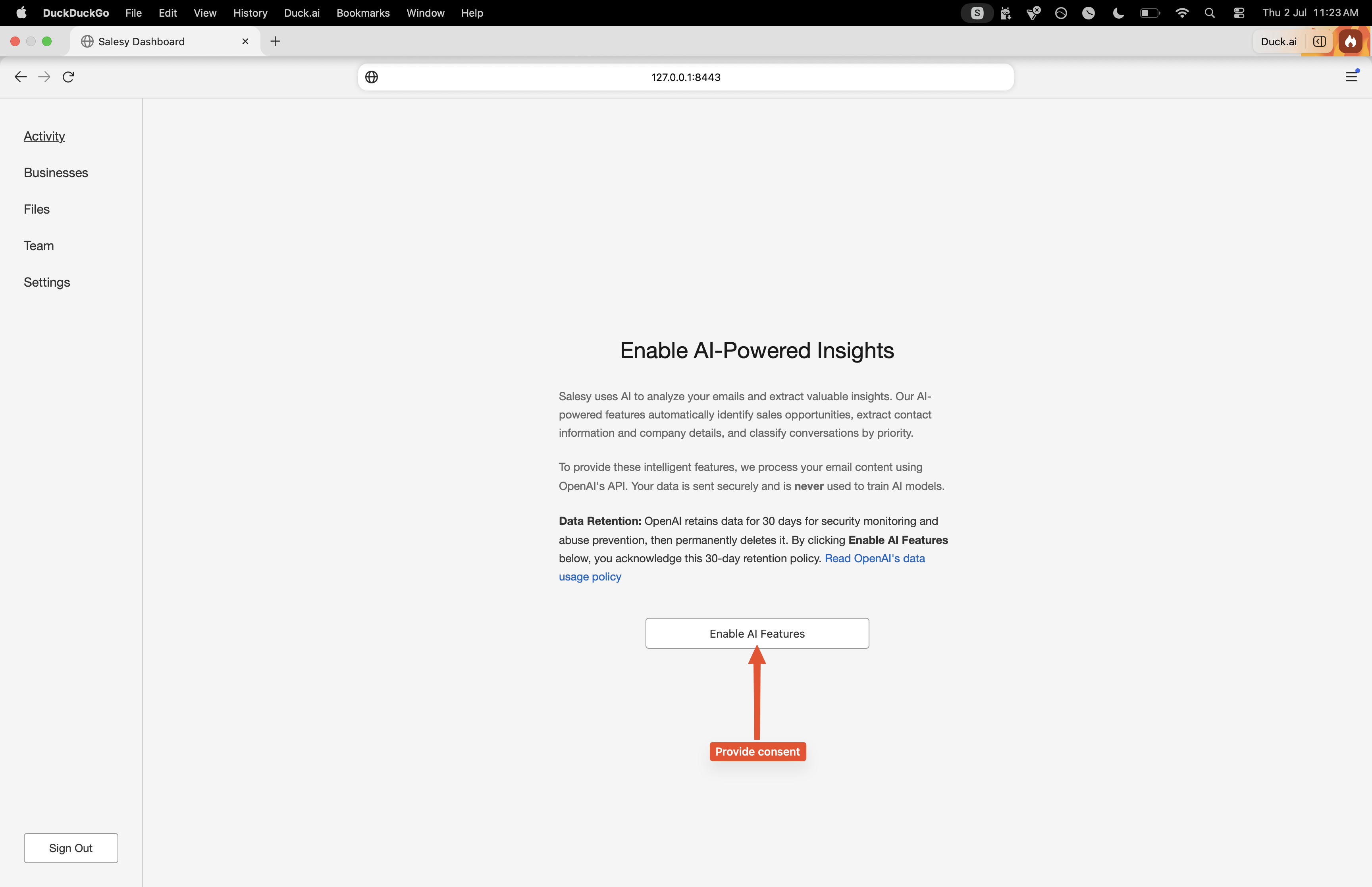
The very first time a user logs into their Salesy account, they’re presented with the consent screen. This is to make them aware of how their data is processed. As of writing, Salesy uses OpenAI’s models for reasoning. This means that the content of user’s email will be sent to OpenAI. By deafult, OpenAI retains the data for a period of 30 days. Their zero data retention policy is only available for enterprises with a qualifying use case. Similarly, another option is to use self-hosted open-source models. The economics of this makes sense when the scale is high enough. For the initial version, it’s only feasible to use hosted models. With this constraint, the user is asked to consent to Salesy’s use of OpenAI and be aware of the retention policy.
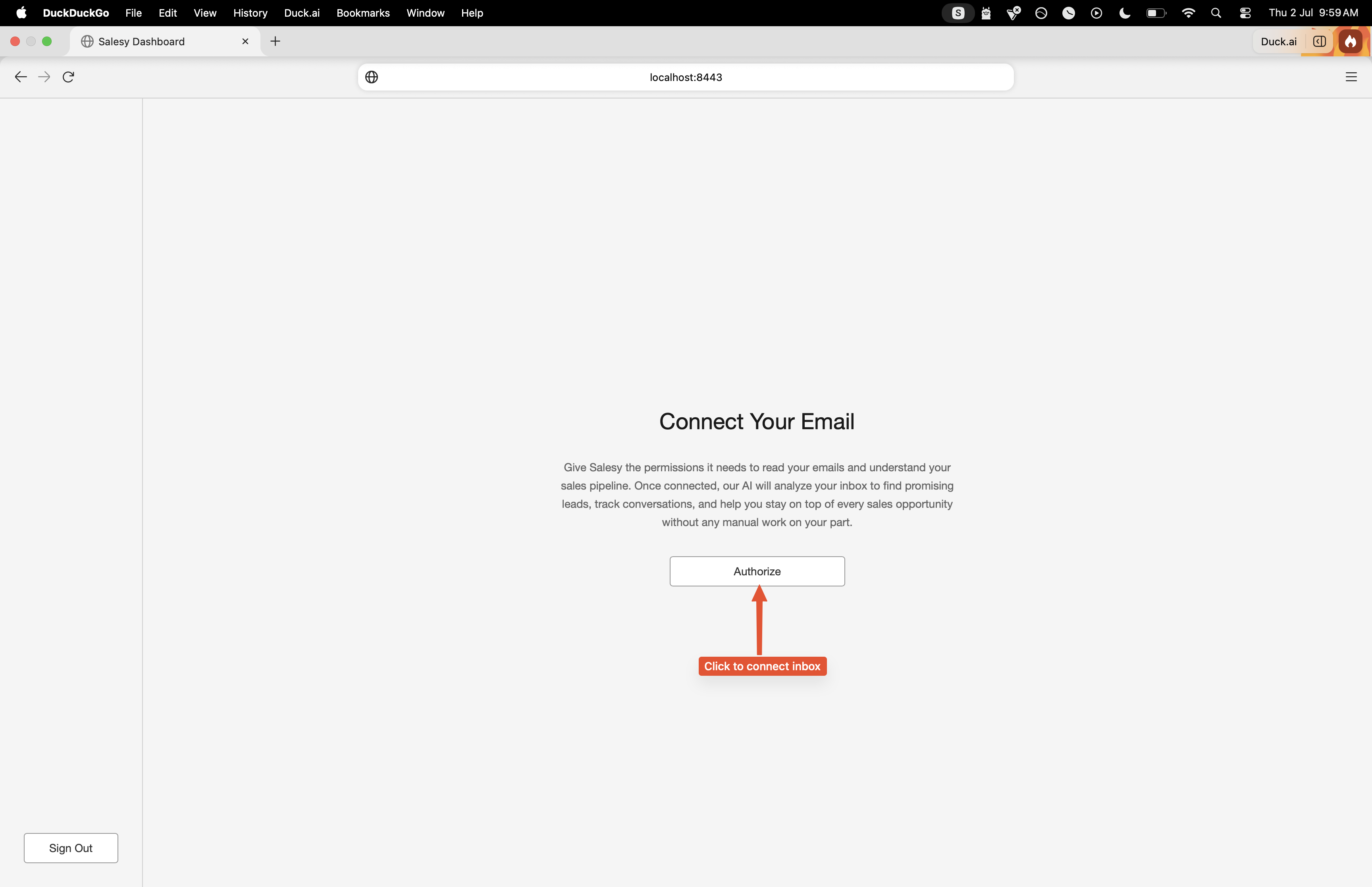
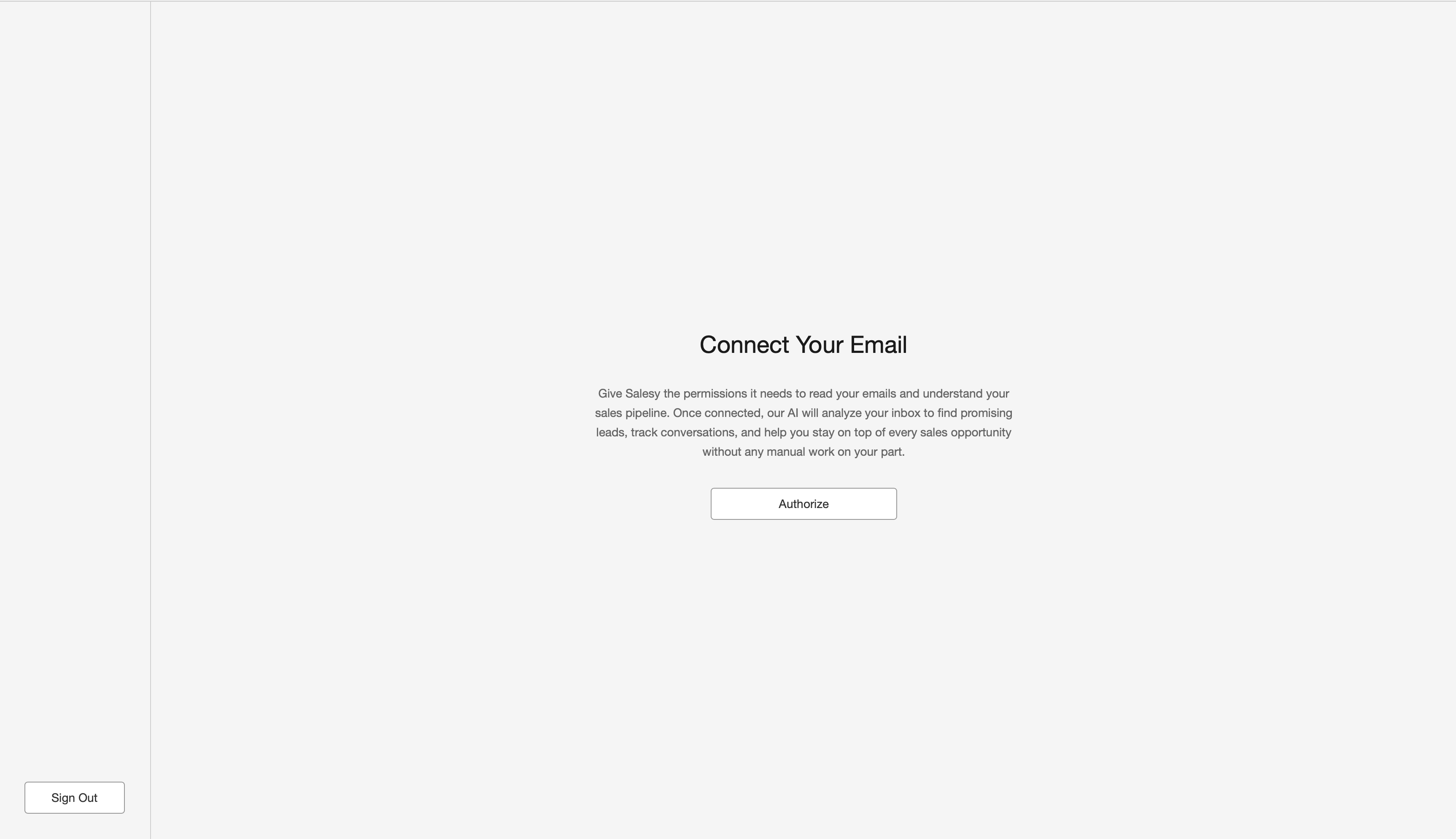
Once the user has consented, they’re presented with the button to connect their inbox with Salesy. For the first iteration, it only works with Gmail. Clicking on the “Authorize” button takes them through the Gmail OAuth process. They’re asked to give Salesy the permissions to read their inbox and to send emails.
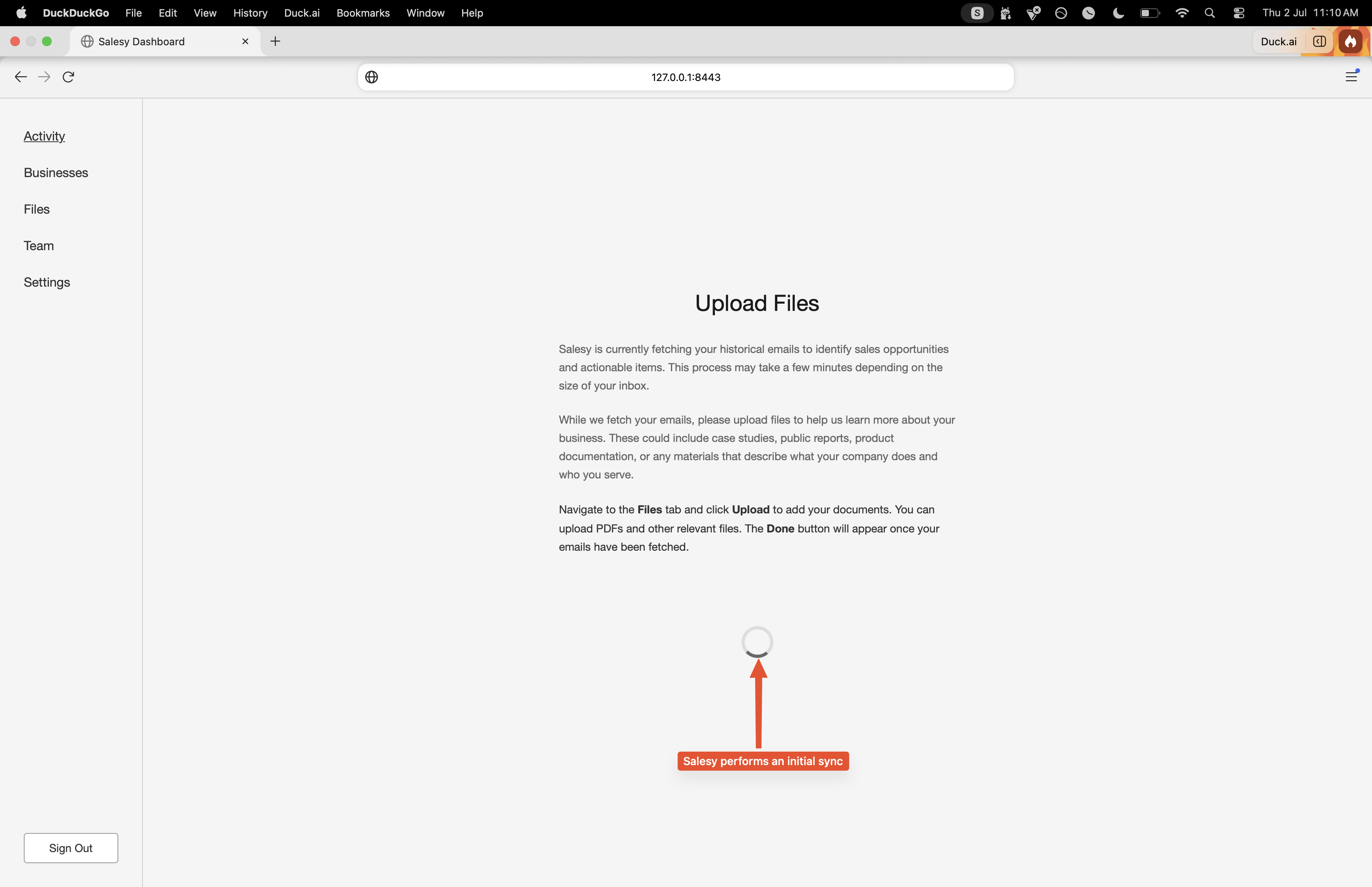
After they’ve connected their inbox by completing the OAuth process, Salesy begins a historical sync of the Gmail inbox. Given that this is a time-taking process, the user is asked to upload files into the system. We’ll look more into what the different types of files can be in a later post. For now, it’s sufficient to know that these can be questionnaires, instructions, general information about the company, and so on.
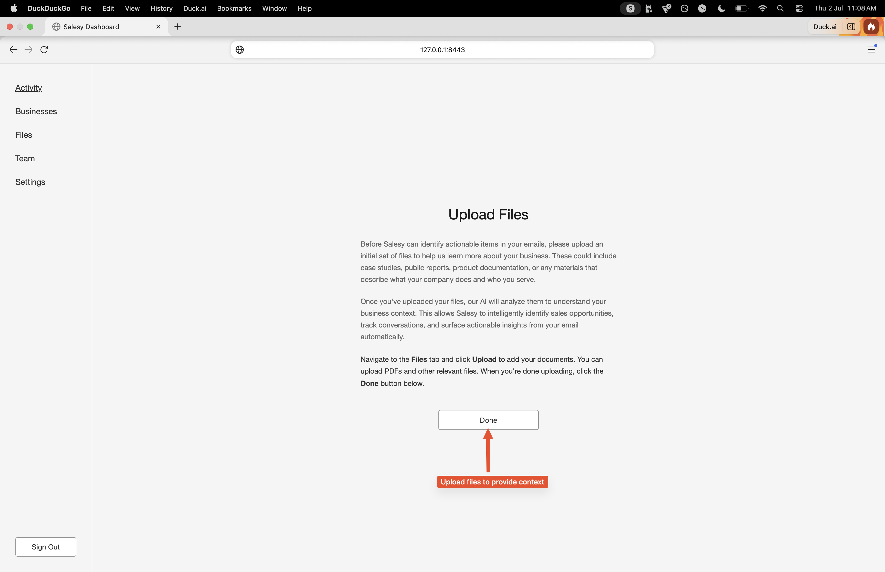
A spinner is presented while the initial sync runs and changes to the “Done” button once it is complete. Once the sync is over and the files have been uploaded, Salesy will begin analyzing the emails and drafting responses to them. While drafting responses, it’ll gather information from the relevant files to ensure that what’s drafted is grounded in information provided by the user.
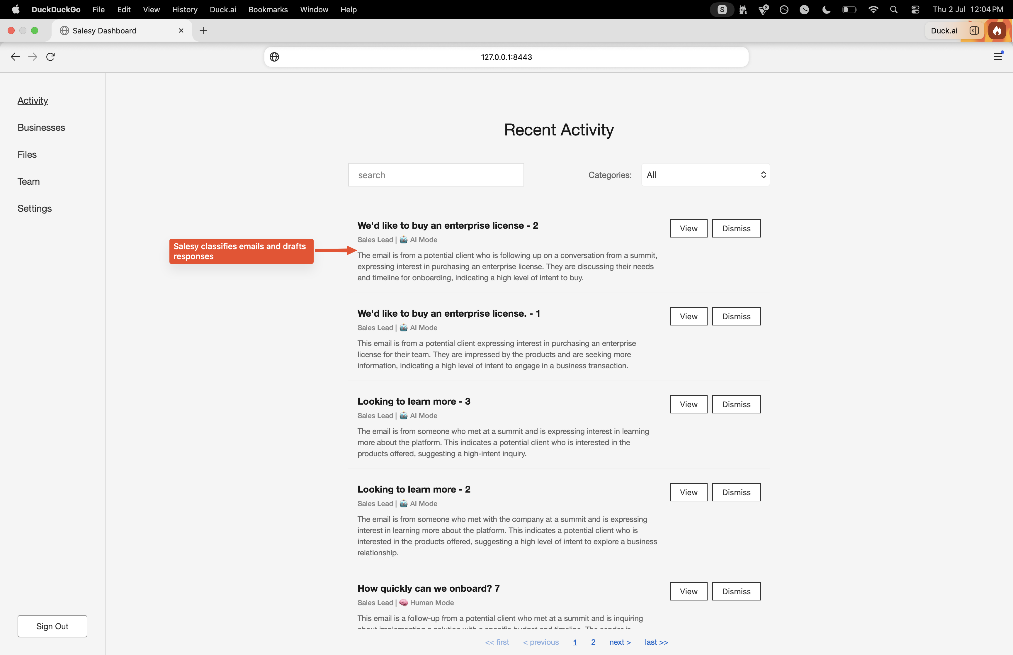
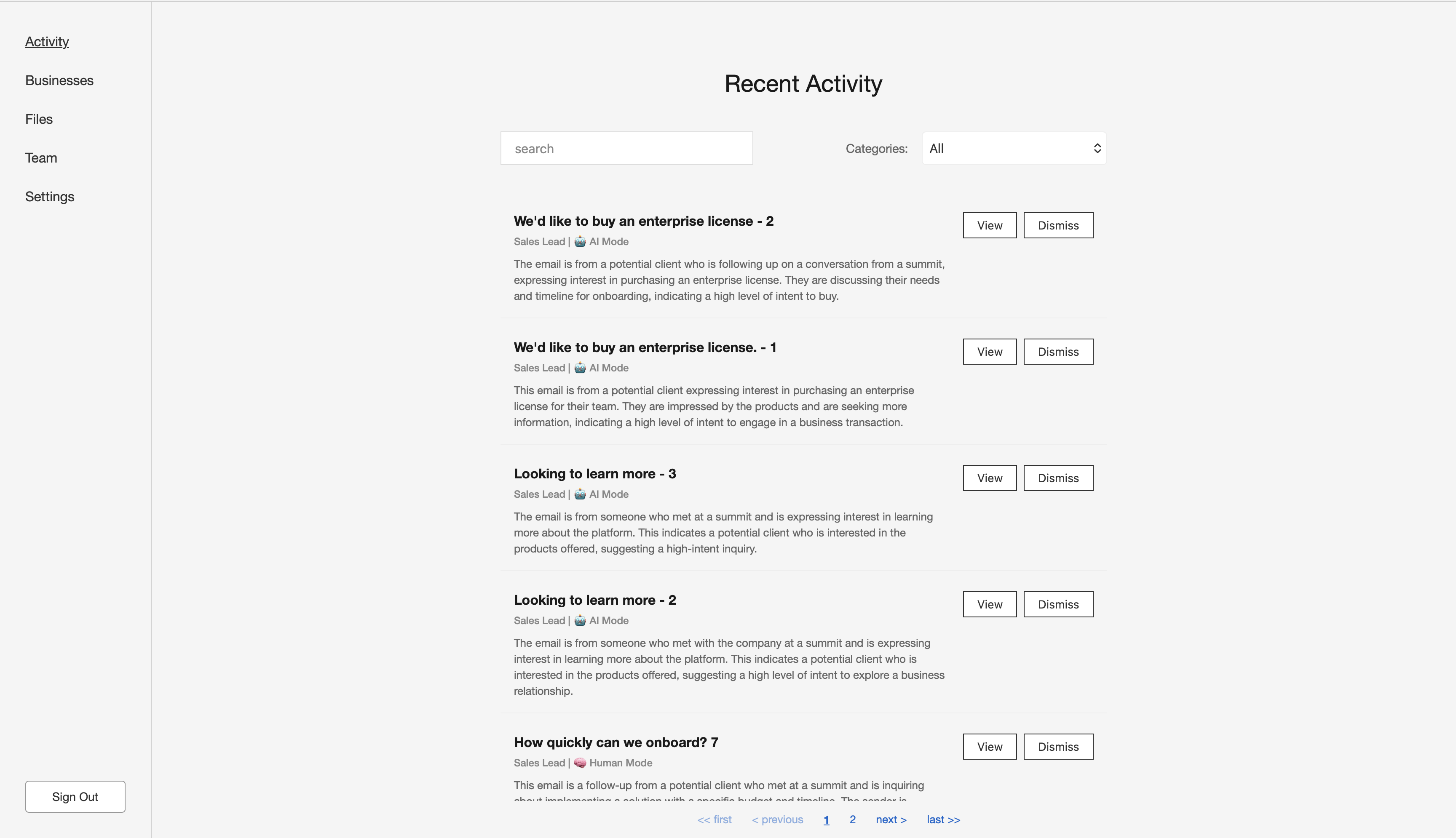
As Salesy drafts each reply, it presents them to the user in the dashboard. Each item in the list is presented with information like its label, such as “Sales Lead”, whether it is human driving the conversation or AI, by mentioning that the conversation is in “AI Mode” or “Human Mode”, and a brief summary of the email. The user then has the option to view the details of the drafted response or dismiss it altogether.
Conclusion
That’s it. That’s how you connect your inbox to Salesy. In the next post we’ll look at how to upload files to Salesy.
Lately I’ve been working on an AI side project that’s an assistant for sales executives. The aim of the project is to automate as much of the sales process as possible by adding AI into the mix. The catalyst behind this project is the observation that there are industries where sales happen over email. Sales executives can connect their inbox to the system, allowing it to handle much of the sales journey automatically while they focus on the more human aspect of the process like relationship building. I nicknamed the project as “Salesy” and this series of posts will walk you through how it is built and what it does. This introductory post outlines some of the features of the project.
Defining the Product
Salesy is a human-in-the-loop AI sales assistant that analyses every incoming email and intelligently guides the prospect through the sales journey. It is a system which automates the sales journey by reading the inbox of the sales executive and allows improving efficiency by handling much of the repetitive work like asking and answering common questions, guiding the prospect through the sales journey, and so on. There is a singular persona that it is designed for — the sales executive.
Defining the Goals
The following are the list of goals for Salesy.
Improve the efficiency of the sales executive by drafting their emails.
Improve the efficiency of the organization by moving prospects through the sales journey seamlessly.
Improve the satisfaction of the prospect by providing them with relevant information when they need it.
The following are the KPIs to be tracked.
The number of emails sent by Salesy.
The number of steps the prospect has moved through and the time spent in each.
The number of questions asked by the prospect to gather information.
The number of questions asked by Salesy to gather requirements.
Constraints and Limitations
There is one major constraint in the system. Anything that happens outside the email thread cannot be captured. A couple of examples demonstrate this. Consider an industry where the prospect may request a sample to be sent before an order is placed. Dispatching the sample and awaiting its delivery happen outside the email thread. A similar constraint is encountered when the prospect requests a meeting, either virtual or in-person. Thus, the system can automate the sales journey only using information that’s present in the ongoing email thread. Any information captured outside the email would need to be added back to it. For example, by sending a follow-up email to capture what was discussed in the meeting.
Features
Connect Email
The first step in using Salesy is to connect the inbox with the system. For the case when the user uses Gmail, they’d have to perform OAuth authorization and give Salesy the permission to read their inbox. As shown in the screenshot above, the prompt tells the user why Salesy needs these permissions and the “Authorize” button begins the OAuth process.
Activity
Once the inbox is connected, Salesy categorizes each incoming email. The “Activity” tab provides an overview of the emails that require the user’s attention. The screenshot above shows the ones that have been labelled “Sales Lead”. Each item in the list shows the title of the email, its label, whether it’s AI handling the conversation or the human since it’s a human-in-the-loop system, and a summary of the email. The user has the option to “View” the details of the action suggested by AI or to “Dismiss” it.
Businesses
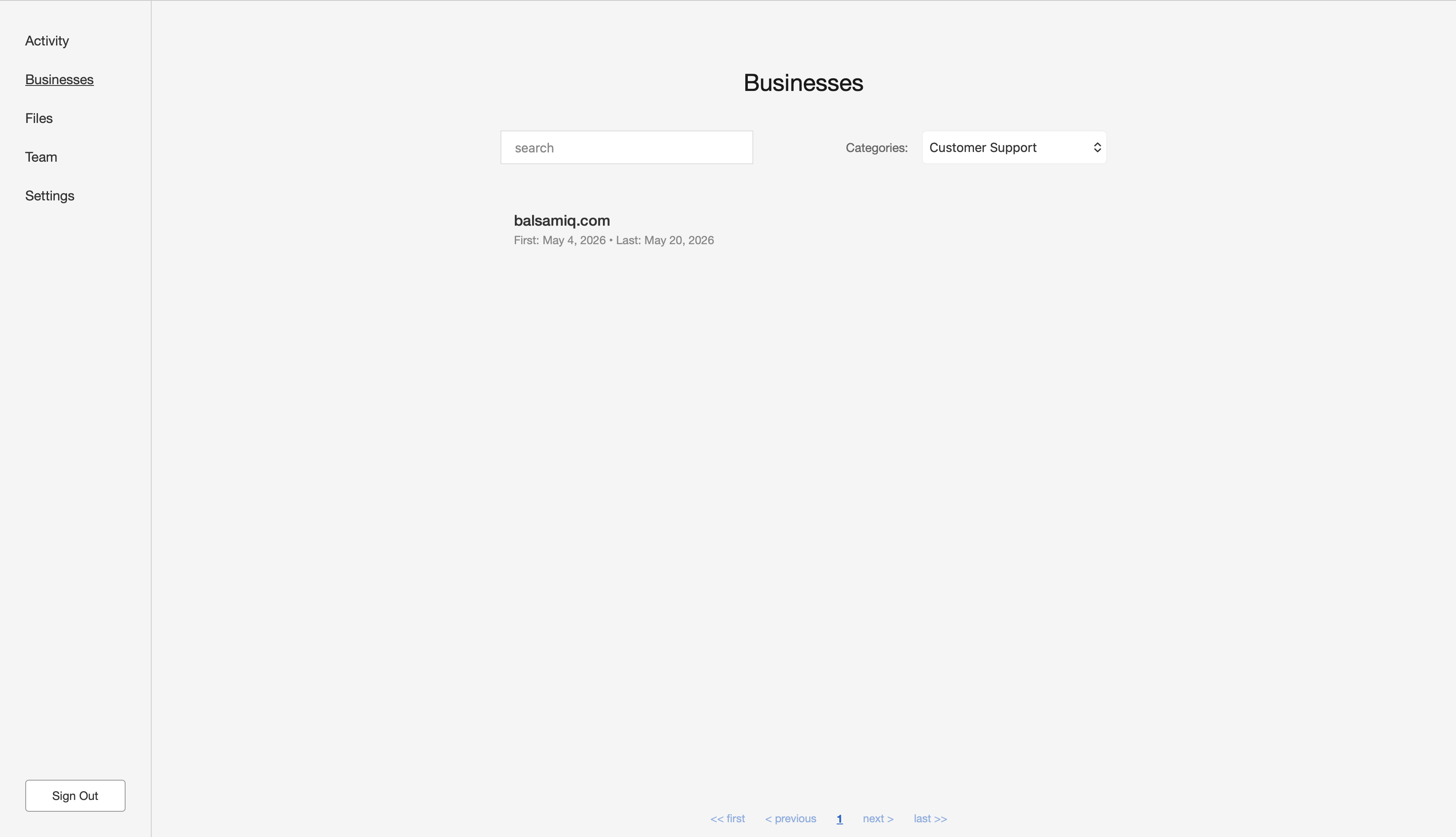
The “Businesses” tab provides a quick way for the user to find out which businesses they are in conversation with and why. That is, who’s interested in making a purchase or requesting after-sales support. Since Salesy is B2B, every business is identified by their domain. Clicking on the domain displays the conversations associated with that business. Additionally, the user is also shown the first and last dates of communication with that business.
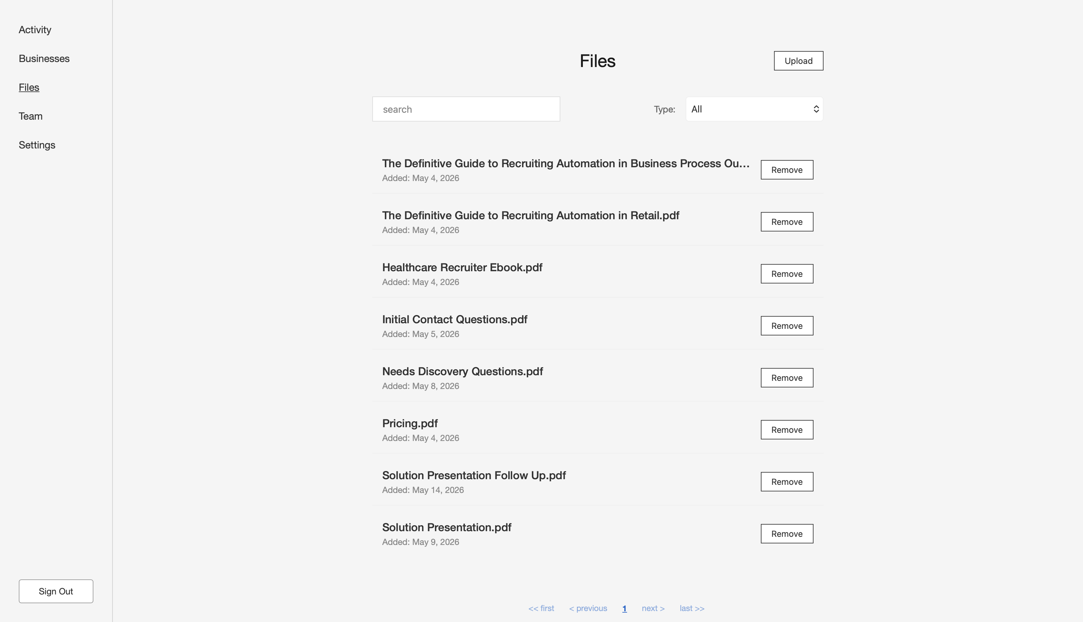
Files
The “Files” tab allows the user to upload files. These are used by Salesy’s AI to construct response to emails. Files can be of different types. For example, you may have one file which contains all the questions the bot should ask to determine the requirements of the prospect and another which contains general information about the company. Some of these files are read in their entirety to construct a response where as others are read in parts as chunks.
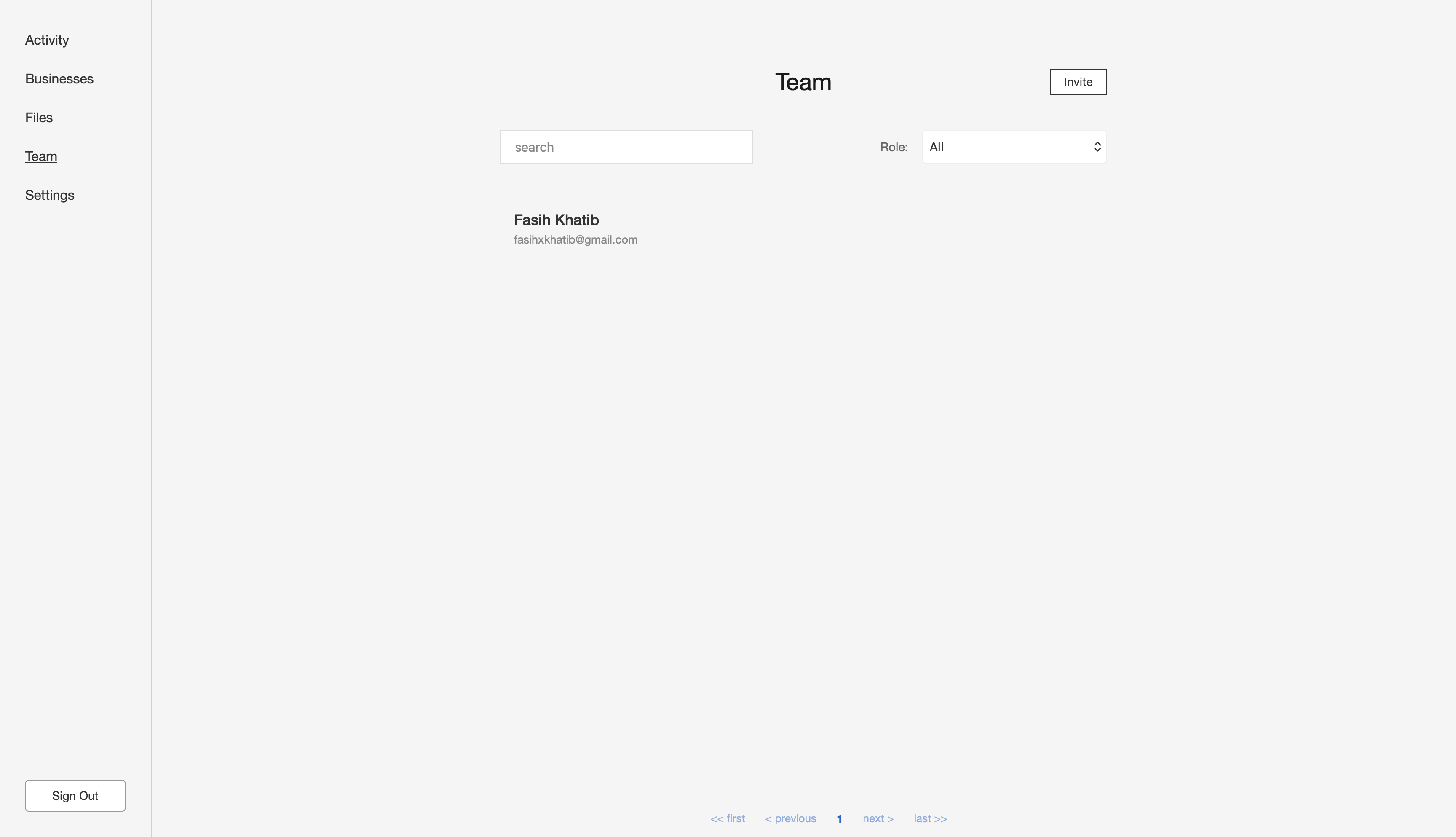
Team
The “Team” tab allows inviting other people to Salesy.
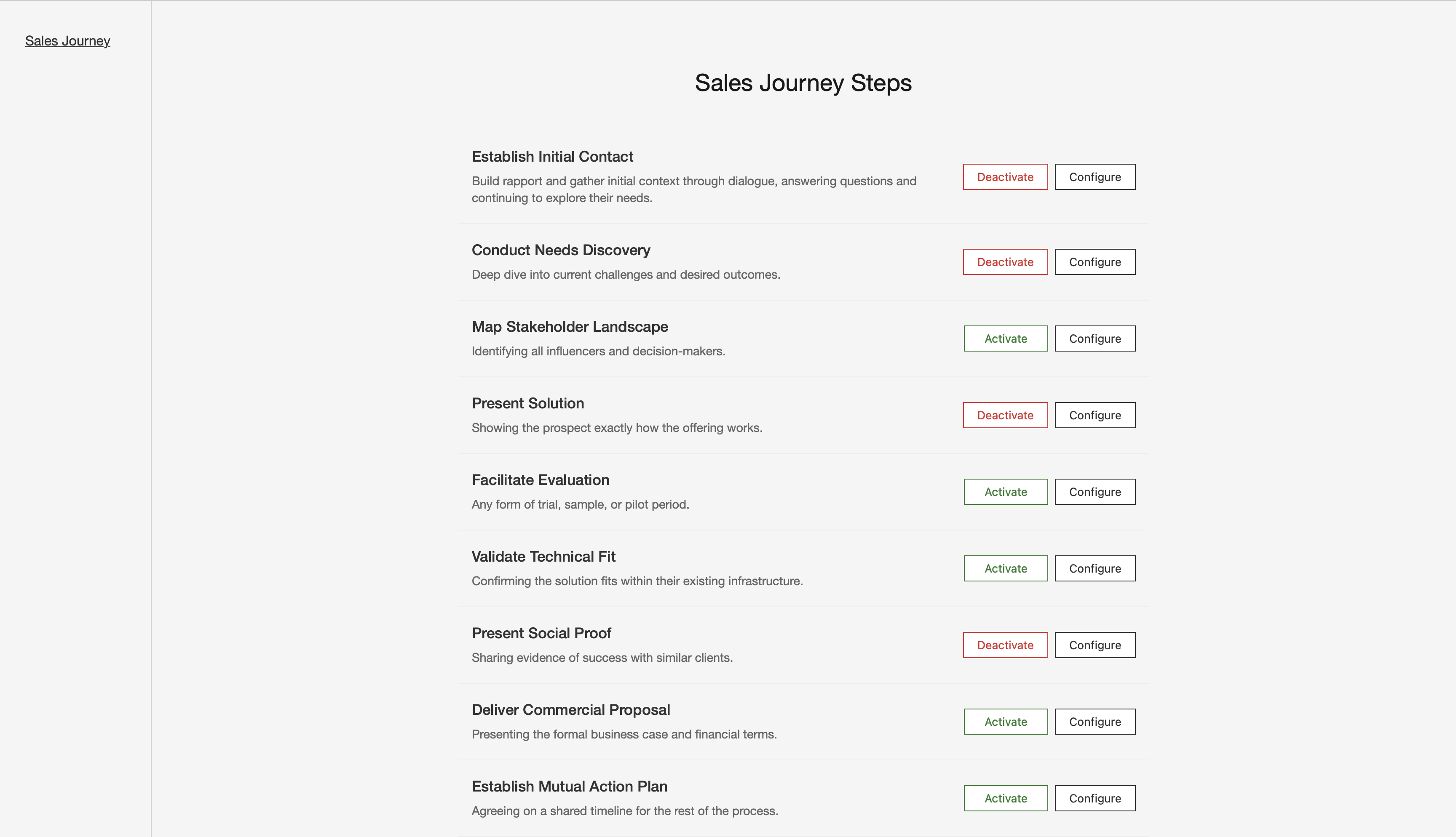
Settings
The “Settings” tab allows changing the settings in the system. For example, since different organizations have different sales journeys, the various steps the prospect goes through can be configured via the settings.
Conclusion
This was a brief overview of what Salesy can do. Starting with the next post, we will look at each of the features outlined above in more detail. Then, subsequent posts will look at the engineering behind the project.
One of my favorite food delivery apps recently launched a feature where they spotlight restaurants. Upon clicking the icon which shows you more about the restaurant, you’re presented with a list of all the outlets they have in the city. As someone who eats outside frequently and eats a variety of different cuisines, this got me thinking. What if we could elevate this experience? While previously I’d written about a feature I’d love to see from a programmer’s perspective, I’ll write this post from a product manager’s perspective. In essence, I’ll attempt to write a Product Requirements Document (PRD). I’ll follow the “How to write a PRD” guide by Notion. Here it goes.
Step 1 - Define the Product.
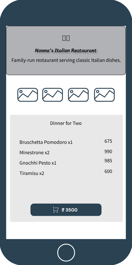
The aim of the product is to elevate a diner’s experience of a restaurant by presenting them with curated menus. Curated menus allow the diners to expreience the best of what the restaurants have to offer by letting them focus more on what makes eating out an experience — the cuisine, the company, and the conversations.
There are various personas who will benefit from such a product. These personas are defined below.
Persona 1 — The Explorer.
People who like eating out frequently and trying new places and cuisines to eat can benefit from handpicked dishes presented in the curated menu. This allows them to experience new tastes and cultures whle enjoying a tailored exprience; every dish in the menu is chosen to delight the diner by highlighting the best of what the culture has to offer.
Persona 2 — The Executive.
Curated menus also make dining in a business setting easier by letting the diners focus more on enjoying the cuisine, and having business discussions than choosing dishes out of a menu. This also allows highlighting, if there are diners from various countries, the cuisine of the host country.
Persona 3 — The Lover.
Curated menus make going out on dates a more memorable experience by allowing partners to bond over meals shared together. The menu takes the mystery out of choosing the right dish as each is chosen to delight the diner. This makes going out and choosing the right restaurant for the evening an easier experience.
Step 2 - Determine Goals.
The following are the list of SMART goals which will enable the release of the first iteration of the product.
Identify the top three cities where users eat out the most.
Identify the five restaurants in these cities who’d participate.
Create three curated menus for each of these restaurants.
Get 100 bookings for each menu in the first six months.
The KPIs for the goals are listed below.
The number of people viewing curated menus.
The number of people buying curated menus.
The number of people adding curated menus to their favorites.
Step 3 — Constraints and Limitations.
Curated menus take time to create. Getting each restaurant onboard, creating the menu, presenting them to the user, and getting them to choose the menu can be a time-taking process. Additionally, factoring in people’s dietary choices mean that some menus will have limited appeal thus reducing the number of people who choose the menu. Another factor is the pricing of the menu requiring them to be created at different price points.
Step 4 — Scope.
The initial pilot of the feature should include only a limited number of restaurants and menus. From the point-of-view of functionality, the engineering effort required should focus on enabling the foals outlined in Step 2 — adding curated menus in the system, displaying them to users, allowing users to buy the menu, notifying the restaurants of the purchase, and analytics to track the KPIs.
Step 5 — Features.
Upon viewing a restaurant, the user will be presented with the list of curated menus for that restaurant along with the price. They will be able to buy it within the app by choosing a date and time, and paying the displayed amount. This will reserve a table for them and notify the restaurant that a curated experience is expected at the chosen time.
Step 6 — Release Criteria.
The criteria for success would include trial runs with restaurants with a chosen group of users and ensuring that the functionality performs as expected. Once past this phase, the feature can be released generally to more users. Concretly, the following criterias would help check the readiness of the product.
Add the participating restaurants into the system.
Add the curated menus into the system.
Ensure that the menus show up in the app as expected.
One of my favorite food delivery apps recently launched a feature where your friends can recommend dishes to you. This got me thinking. What if we could provide recommendations from more than just friends? What if recommendations came from the people around you as they browse restaurants and place orders? In this post we’ll take a look at how we can go about building such a system.
Getting Started
Imagine opening your favorite food delivery app and being presented with the trending searches and restaurants. For example, something like the mockup shown below. It shows three trending searches and a few trending restaurants. It turns out that by tracking user activity from search to purchase allows us to find out what’s gaining traction. Let’s design such a system.
We’ll begin by tracking a user’s journey from search to purchase.
Let’s say that the user begins their food ordering journey by searching for “pizza”. They’re presented with a list of restaurants that sell pizza. They click on a few restaurants, browse the menu, and finally add a large pizza to their cart from one of the restaurants. Finally, they place the order by making the payment. If we were to track each interaction of the user as an event, it would look something like this.
Search for “pizza”. Present a list of restaurants. Click on a restaurant. Click on a restaurant. Add pizza to cart. Add a bottle of cola to cart. Purchase.
As we collect more events, we’ll see patterns emerge. For example, we may discover that pizza is one of the trending searches since it’s being searched more often. Let’s see how we can do all of this programatically. It all starts with tracking the user’s search.
Let every search generated by the user be tagged by a unique identifier. This identifier, which we’ll call query_id, will be unique throughout the journey. Every new search will generate a new query_id but will stay unchanged for the same search. Similarly, we’ll track a user with a unique identifier called user_id. Let’s model the user’s search as an event as follows.
In this event, which is of type “query”, the user searched for “large pizza”. Similarly, we’ll model the results that were displayed to them as an event.
In this event, which is of type “results”, we see that the user was presented with two restaurants. Next, let’s model the user clicking on one of the restaurants.
In this event, which is of type “click”, the user clicked on the restaurant called “La Pizzeria”. Next, let’s model the user adding two items to their cart.
In the events, which are of type “purchase”, we see that the user purchased the two items.
Having seen how to track user journey from search to purchase using events, let’s see how we can mine these events for patterns. Let’s write a simple Python script which demonstrates this using the events we’ve seen above.
query item count 0 large pizza 16 inch Margherita 1 1 large pizza Cola 1L 1
In the output, we see that the query “large pizza” resulted in the purchase of one pizza and one bottle of cola.
What the script does is tie the purchase to its original query using the query_id. Finding the trending phrases and keywords is now simply a matter of grouping on the query.
This gives us the following output which shows us that the query “large pizza” resulted in the purchase of two items.
1 2
query count 0 large pizza 2
As we collect more events, we’ll see more query phrases emerge. These can then be presented to the user in the application. Similarly, tying the click events to queries will show us what query phrases bring the user to a particular restaurant. Finally, aggregating the click or purchase events will show us which restaurants are trending.
This small example shows how tracking user interactions with events can be used to find which query phrases are trending.
In a more production environment, and to make this real-time, events would have to be emitted to a log like Kafka and processed with a stream processing framework like Spark or Flink. Once these aggregated metrics are generated, they’d be written to some database from where they can be served to the user.
In the previous post we saw how we can embed a Superset dashboard in a webpage using a Flask app. In this post we’ll look at creating indexes on the tables that are stored in Pinot. We’ll look at the various types of indexes that can be created and then create indexes of our own to speed up the queries.
Getting started
Very briefly, a database index is a data structure that improves retrieving data from the tables. It is used to quickly find the rows that we’re interested in without having to scan the entire table. Pinot supports different types of indexes that can be used to speed up different types of queries. Knowing the access patterns of the queries helps us decide which indexes we’d like to create. We’ll quickly look at each type of index that Pinot provides, write a few queries, and then create indexes to speed them up. Let’s start by looking at the various index types that are available in Pinot.
Pinot supports the following types of indexes — bloom filter index, forward index, FST index, geospatial index, inverted index, JSON index, range index, star-tree index, text search index, and timestamp index. In the sections that follow, we’ll look at how to create an inverted index, and a range index to speed up our queries. Let’s start with the inverted index.
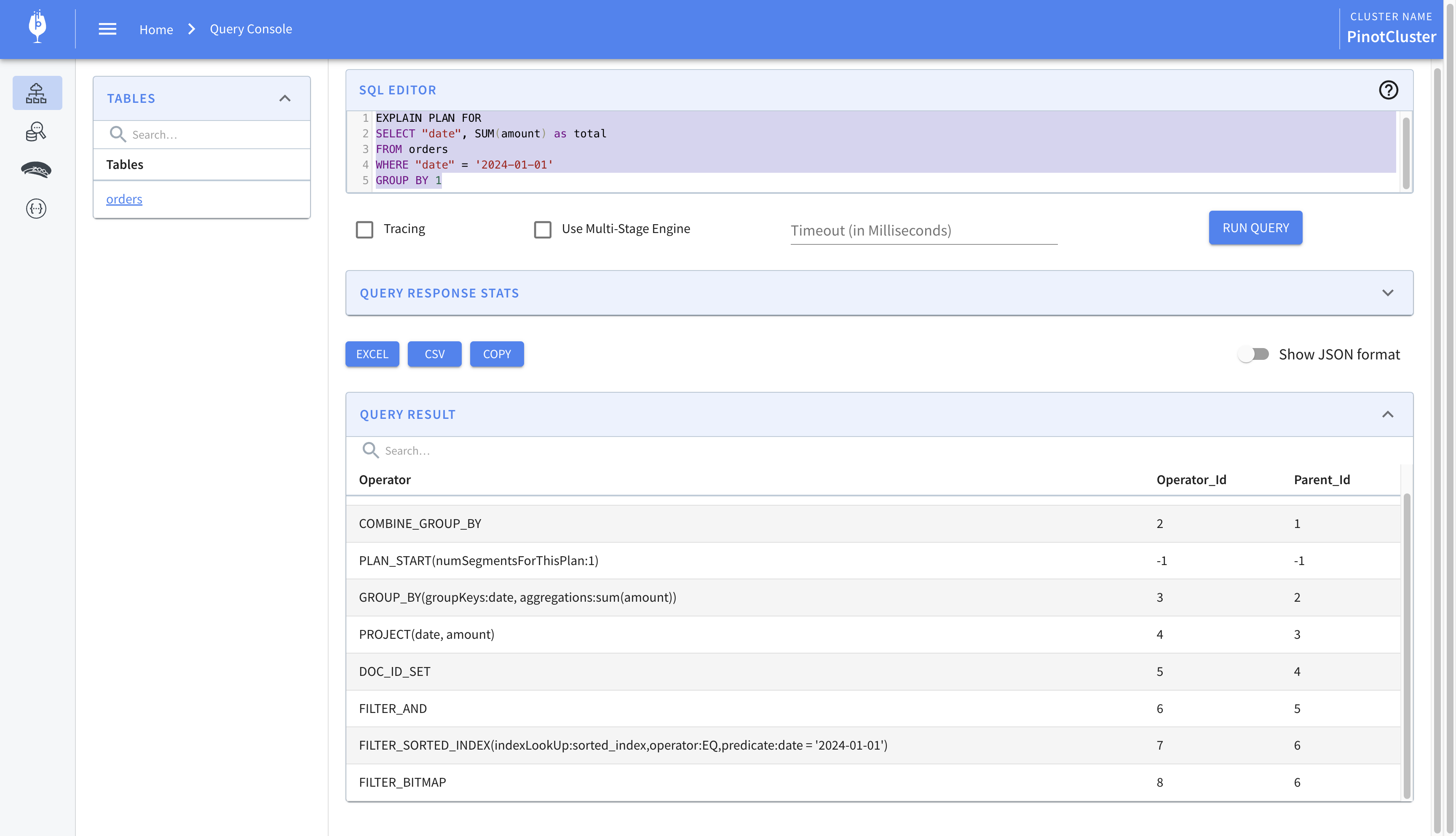
Let’s say we’d like to find out the sum of the amounts of orders placed on January 1st. One way to write this query would be to convert the created_at time to a date on the fly. This would require us to look at every row we have in the table and compare it against the date we’re looking for. Another way to write this query would be to convert created_at to a date during ingestion time and create an inverted index on it. Creating an inverted index would store a mapping of each date to the row IDs with the same date. This will enable us to filter only those rows which have the date we’re looking for instead of having to look at each one of them.
We’d have to update our table and schema for the orders table. We’ll start by adding a column to our schema definition which will store the date as a string.
1 2 3 4
{ "name":"date", "dataType":"STRING" }
Next, we’ll convert the created_at time to a date and store it in the date column. To do this, we’ll create a field-level transformation in the table definition.
Let’s modify the query slightly and look for the daily total for the last 90 days. It looks as follows.
1 2 3 4 5
SELECT "date", SUM(amount) as total FROM orders WHERE created_at >= ago('P90D') GROUPBY1 ORDERBY1
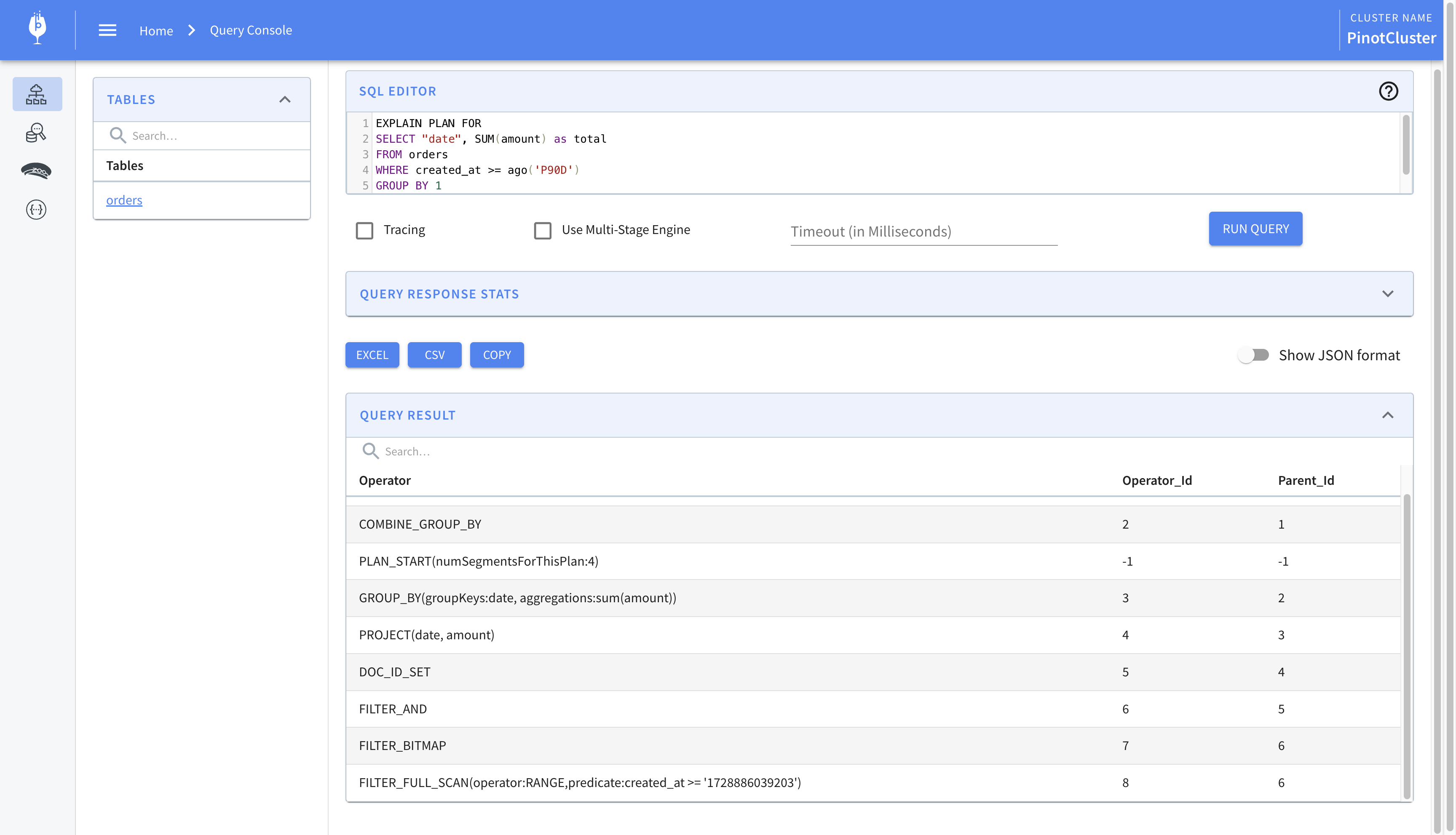
The ago() function takes as argument a duration string and returns milliseconds since epoch. We compare it against created_at, which is also expressed as milliseconds since epoch, to get the final result. Let’s look at the explain plan for the query.
We find the following line which indicates that an index was not used.
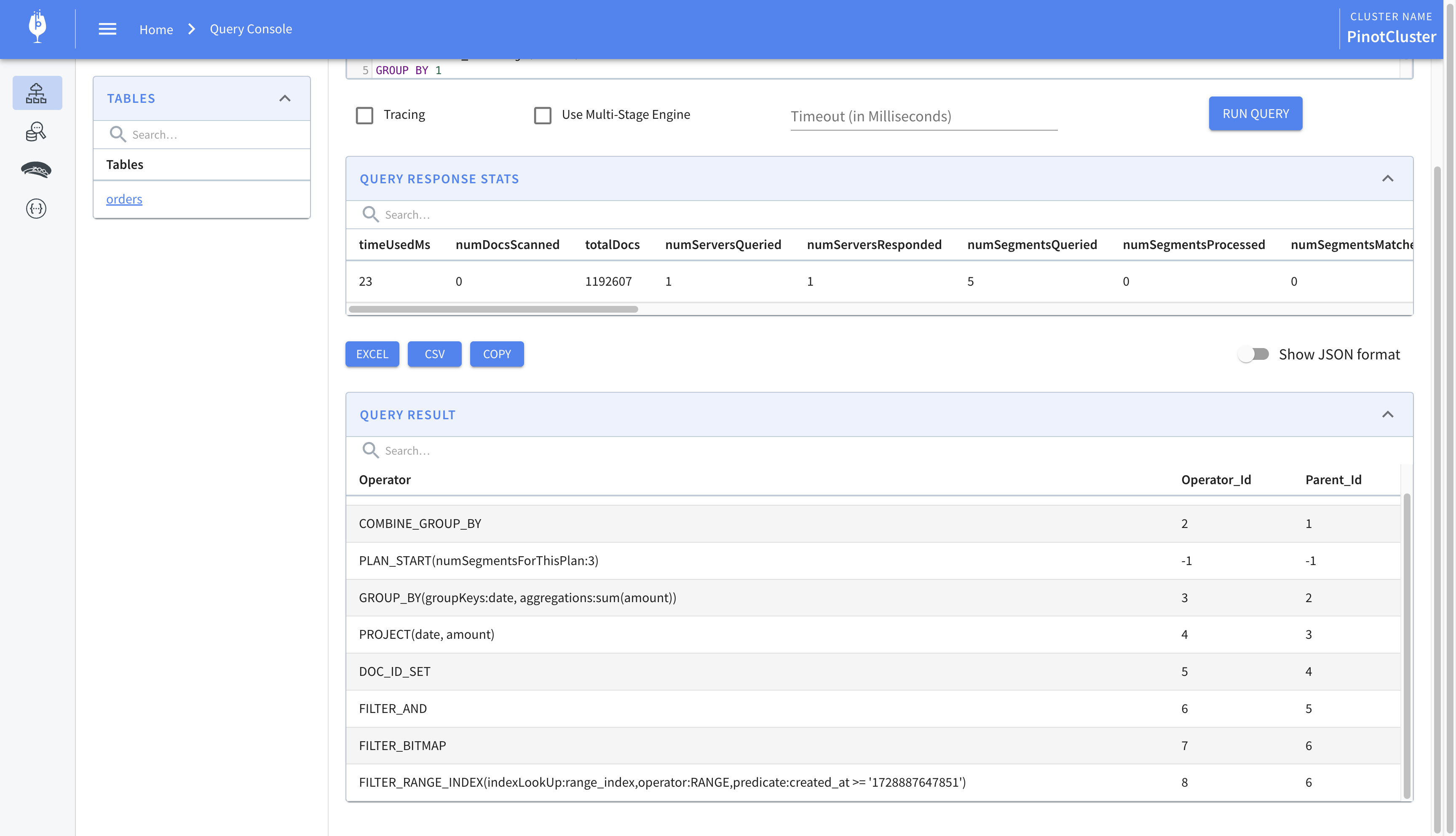
We can improve the performance of the query by using a range index which allows us to efficiently query over a range of values. This helps us speed up queries which involve comparison operators like less than, greater than, etc. To create a range index, we’ll have to update the table definition and specify the column on which we’d like to create the index. We’ll add the following to the table definition.
This was a quick overview of using indexes to speed up queries on Pinot. We looked at the inverted index and the range index. In the next post, we’ll look at the star-tree index which lets us compute pre-aggregations on columns and speeds up the result of operations like SUM and COUNT. We’ll also look at stream processing to generate new events from the ones emitted by Debezium.
In the previous post we looked at how to visualize our data using Superset. In this post we’ll look at embedding our dashboards. Embedding allows us to display a dashboard outside of Superset and within a webpage. This lets us blend analytics seamlessly into the user’s workflow. We’ll tweak a few Superset settings to allow us to embed a dashboard, and then build a Flask application which will render it in a webpage. We’ll also look at row-level security which lets us limit a user’s access to only those rows that they are allowed access to.
Getting started
Let’s say we’d like to create a dashboard that consists of a line chart and a table. The line chart plots the number of orders the user has placed daily. The table shows the cafes where the user frequently orders from. We’ll start by writing a query which will enable us to create the line chart. This will be stored as a view so that rendering the data produces realtime results. The query is as follows.
1 2 3 4 5 6
CREATEVIEW hive.views.daily_orders_by_users AS SELECT user_id, CAST(FROM_UNIXTIME(CAST(created_at ASDOUBLE) /1e3) ASDATE) AS dt, COUNT(*) AS count FROM pinot.default.orders GROUPBY1, 2;
Next, we’ll create the view which will tell us the cafes the user orders from. It is as follows.
1 2 3 4 5 6 7 8 9 10
CREATEVIEW hive.views.frequent_cafes AS SELECT o.user_id, c.name AS cafe, COUNT(*) AS count, RANK() OVER(PARTITIONBY o.user_id ORDERBYCOUNT(*) DESC) AS rank FROM pinot.default.orders AS o INNERJOIN pinot.default.cafe AS c ONCAST(o.cafe_id ASVARCHAR) = c.id GROUPBY1, 2 ORDERBY1ASC, 3DESC;
Once the views have been constructed, we can use them in Superset to build our dashboard. To enable dashboard embedding, we must first update some Superset settings. If you have any Superset containers running from the last post, start by shutting them down. Then, run the following command to remove any Docker images linked to Superset; we’ll rebuild it with the new settings.
Let’s begin editing the settings. Navigate to the superset directory within the superset repository and open the config.py file. This contains the configuration that will be used by the Superset application when it runs. We’ll edit this line-by-line and see why these changes are required. First, we’ll disable the Talisman library used by Superset. Find the variable TALISMAN_ENABLED and update it to the following.
1
TALISMAN_ENABLED = False
Talisman is a Python library that protects Flask against some of the common web application security issues. Since we’ll be running this locally over HTTP, we can disable this to allow the embedded dashboard to render within the webpage. Next, we’ll disable CSRF protection. Again, all of these settings are to make things run locally over an HTTP connection. You should let these be for production deployment. Find the variable WTF_CSRF_ENABLED and set it to False.
1
WTF_CSRF_ENABLED = False
Next, enable dashboard embedding. This is disabled by default. Find the EMBEDDED_SUPERSET variable and set it to True.
1
"EMBEDDED_SUPERSET": True
Finally, we’ll elevate the permissions of the Guest user to enable us to render dashboards in an iframe. Set GUEST_ROLE_NAME to Gamma.
1
GUEST_ROLE_NAME = "Gamma"
Superset has some predefined roles with permissions attached to them. The Gamma role is the one for data consumers and has limited access. Assigning the Gamma role to the guest user lets us embed the dashboard within a web application. As we’ll see shortly, we’ll generate a guest token which we’ll use when embeding a dashboard.
With these changes made, we can rebuild the Superset images. Run the following command to build them.
This will take a while to build. In the meantime, we’ll start writing our Flask application. It’ll be a simple application that renders a Jinja template. In that template we’ll add the code to display the embedded dashboard. Let’s see what the template looks like.
<style> body, div { width: 100vw; height: 100vh; } </style>
<divid="chart"></div>
<scriptsrc="https://unpkg.com/@superset-ui/embedded-sdk"></script> <script> supersetEmbeddedSdk.embedDashboard({ id: '{{ chart_id }}', supersetDomain: 'http://192.168.0.103:8088', mountPoint: document.getElementById("chart"), fetchGuestToken: () =>"{{ guest_token }}", dashboardUiConfig: { hideTitle: true }, iframeSandboxExtras: [] }) // This is a hack to make the iframe bigger. document.getElementById("chart").children[0].width="100%"; document.getElementById("chart").children[0].height="100%"; </script>
Let’s unpack what’s going on. The embedded dashboard is rendered within an iframe and we need a container element to hold it. This is what the div is for; it’ll hold the iframe.
Next, we load the Superset embed SDK from the CDN. This make the supersetEmbededSdk variable globally available. We call the embedDashboard method on it to embed the dashboard. This method takes an object which contains the information needed for embedding. The first piece of informaton we pass is the id of the chart. As we’ll see shortly, we get this from the Superset UI. We’re using a template variable here and we’ll replace it with its actual value when we render the webpage.
Next, we specify the address of our Superset instance in the supersetDomain field. Here I’ve used the IP address of my local machine to point to the Docker containers running Superset.
Next, we specify the mount point. The mountPoint is the element within the page where the chart will be rendered. We’re retrieving the div using its ID.
Next, we specify the fetchGuestToken function. This function retrieves the guest token from the backend. Since we’re rendering the template from a Flask application, we’ll fetch the guest token on the servier side. Therefore, we simply return the guest token from the function. We’ve used a Jinja variable guest_token which we’ll replace with its actual value when we render the template.
Next, we specify some configuration information. In our example, we’ve hidden the title of the dashboard.
Finally, we increase the size of the iframe so that it fills the screen.
Having written the template, we’ll move on to writing the Flask web application. It’s a single file with one endpoint to render the chart. We’ll write functions to see how we can log into Superset using its API and then fetch a guest token. The complete code for the app is given below.
if __name__ == "__main__": app.run(host="0.0.0.0", port=5555, debug=True)
Let’s step through the code. The chart_id is the unique identifier for the chart we’re trying to embed. As we’ll see shortly, this comes from the Superset UI.
Next, we define the get_access_token function which retrieves an access token. To get this, we need to log into Superset. We use the default username and password which we POST to the login endpoint and extract the token from the JSON that’s returned. This token lets us fetch a guest token which is required for embedding the dashboard.
Next, we define the get_guest_token function which retrieves the guest token. It takes the ID of the user as an argument so that it can apply row-level security to the dataset that powers the dashboard. Row-level security, often abbreviated as RLS, is a mechanism which restricts a user’s access to only those rows that they have the permission to access. If we look at the view we’ve created, it contains the data for all the users. Applying row-level security allows us to display only those rows which pertain to the given user. The rls field in the JSON body contains the clause which limits the access of the user. It is applied as a part of the WHERE clause and filters the rows in the dataset. The resources field contains the ID of the chart that we’d like to embed. The user field contains the details of the guest user.
Next, we define the chart function which actually renders the tempalte. The template is rendered by calling the render_template function which takes the guest token and chart ID as arguments. This generates the final HTML which is returned to the user.
We’ll run this app in a separate terminal by executing the following command.
1
python run_app.py
After waiting for a while to let the Superset images build, we can go ahead and bring up its containers.
1
TAG=4.1.1 docker compose -f docker-compose-non-dev.yml up -d
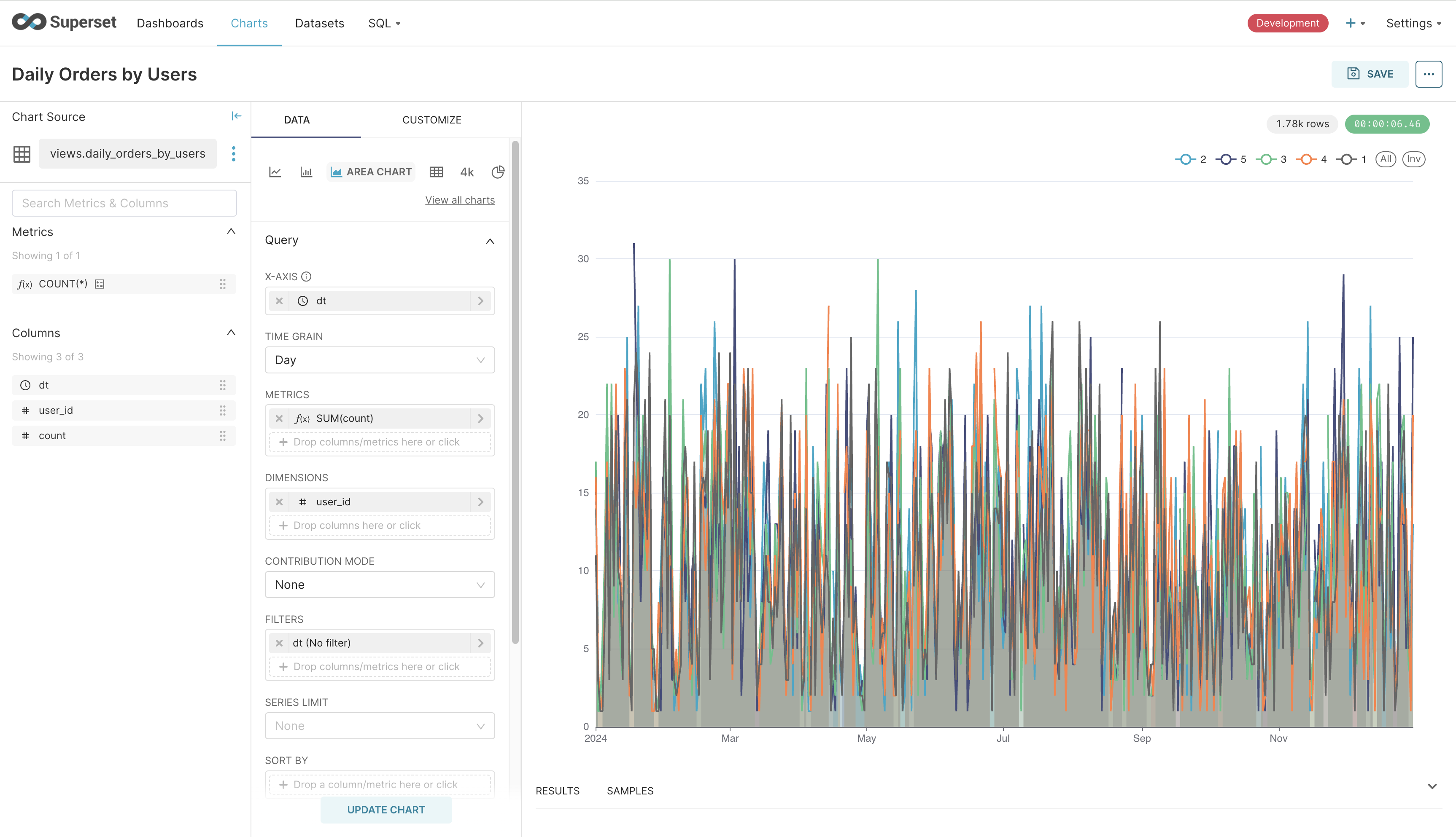
After opening the Superset UI, we’ll begin by creating a dashboard. We’ll add a chart to the dasboard which is backed by the daily_orders_by_users view which we created earlier. We’ll add an area chart where we have date on the x-axis and the count on the y-axis with the ID of the user being the dimension. The screenshot below shows what it looks like.
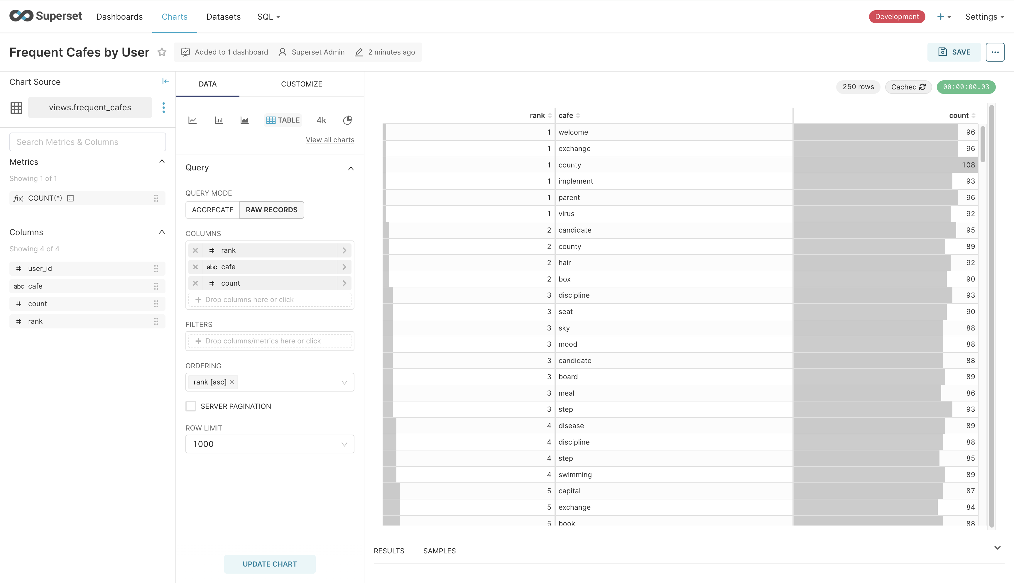
The chart looks cluttered because it is displaying the data of every user. When we embed this chart, we’ll rely on row-level security to display the chart that only belongs to a particular user. Similarly, we’ll add a table backed by the frequent_cafes view and display it in the dashboard. Remember that the filtering is applied to the dataset backing the chart. This means that we can create the table and exclude the user_id column from display.
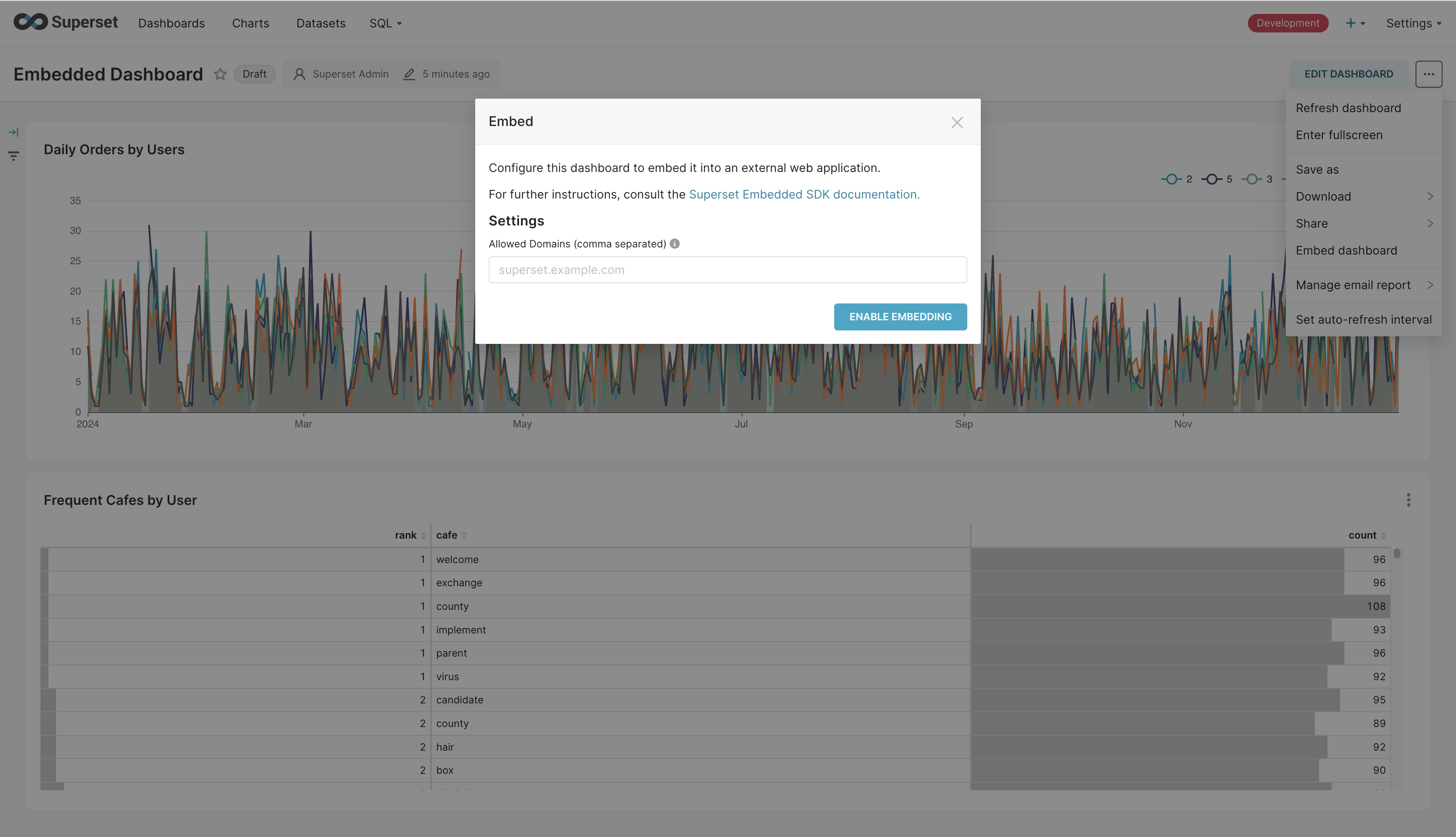
Having added all our charts to the dashboard, we can embed it in the webapp. Begin by saving the dashboard. Then, click on the three dots on the top-right hand and click “Embed dashboard”. You should see a dialog box pop up which allows you to list the domains from which the embedded dashboard can be accessed. We’ll leave this empty to allow embedding from all domains and click “Enable Embedding”. From the next dialog box, we’ll copy the ID of the dashboard and then click the X button on the top-right hand to close it.
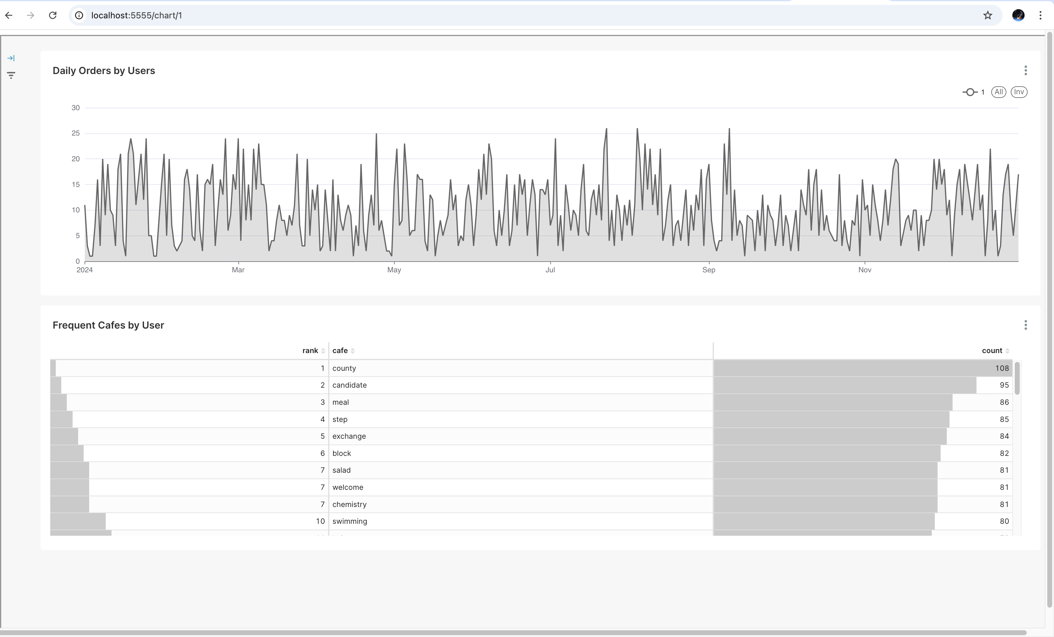
We’ll replace the chart_id variable in our web application and then run it. It will start a Flask application that listens on port 5555. We’ll navigate to http://localhost:5555/1 which will display the chart and the table for the user with ID 1. The embedded dashboard will apply the row-level security clause for this user ID and only display their data. The dashboard looks as follows.
That’s it. That’s how to embed a Superset dashboard.
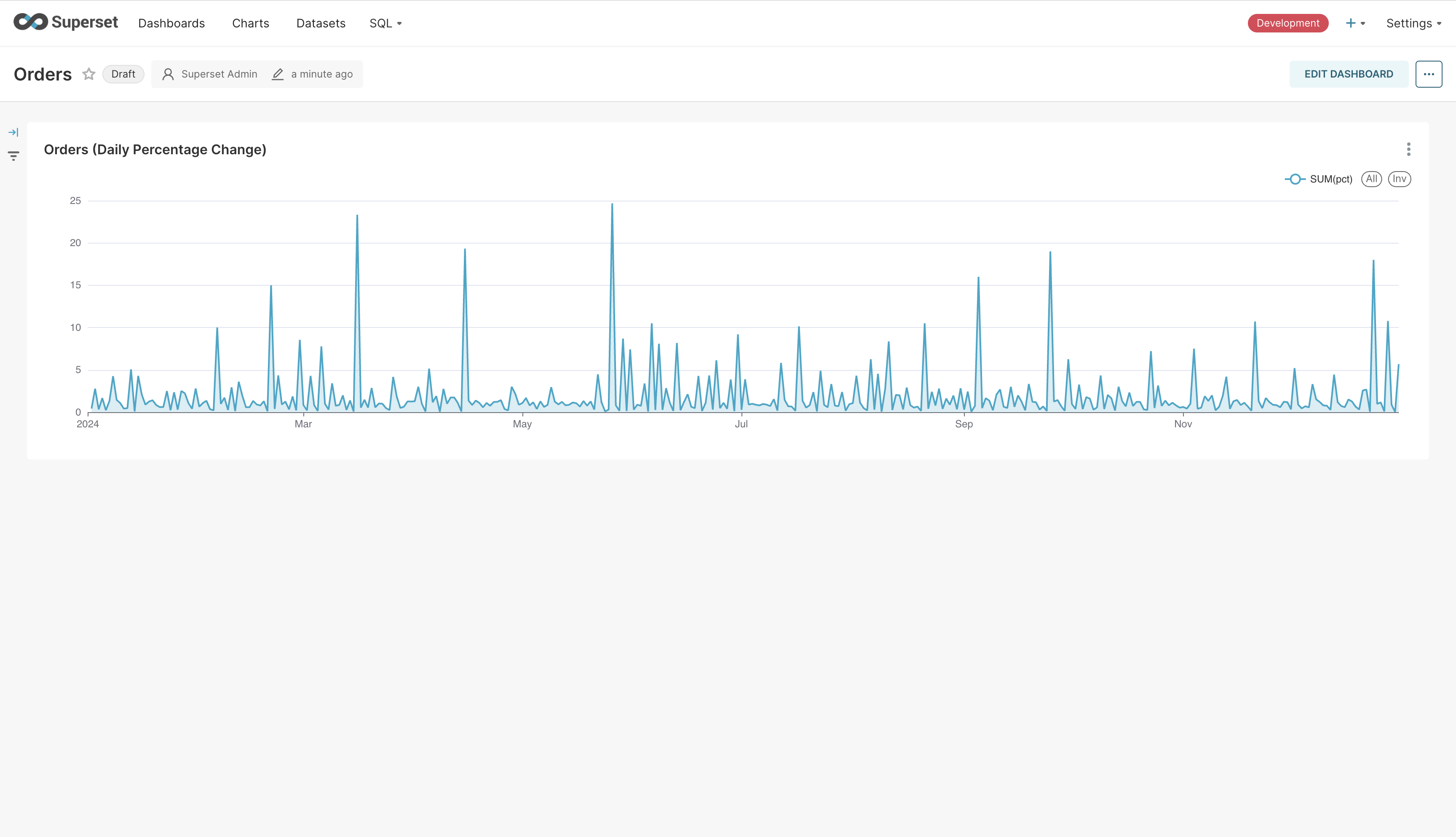
In the previous post we saw how we can use Airflow to create datasets on top of the data that’s stored in Pinot. Once a dataset is created, we may need to present it as a report or a dashboard. In this post we’ll look at how to use Superset to create visualizations on top of the datasets that we’ve created. We’ll create a dashboard to display the daily change in the number of orders placed each day.
Getting started
In an earlier post I’d written about how to run Superset locally. In a nutshell, running Superset using Docker compose requires cloning the repository and checking out the version of the project you’d like to run. In that post I’d also shown how to install additional packages so that we can add the ability to connect to another database. For the sake of brevity, I’ll simply repeat the steps here and refer you to the earlier post for more details.
Let’s start by cloning the repo and navigating to it.
1 2
git clone https://github.com/apache/superset.git --depth 1 cd superset
Next, we’ll checkout the git repository to a specific tag so that we can build from it.
1
git checkout 4.1.1
Next, we’ll add the Python package which will let us connect to Pinot.
1
echo "pinotdb" >> ./docker/requirements-local.txt
Finally, we’ll bring up the containers for this specific tag.
1
TAG=4.1.1 docker-compose -f docker-compose-non-dev.yml up -d
This will build the Docker images for Superset and run them as containers. Once the containers are running, Superset will be available on http://localhost:8088. You can use admin as both the username and password to log in. Now that we’re logged in, we can begin creating charts and dashboards. Let’s start by connecting to Trino.
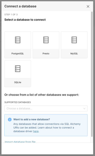
Click on “Settings” on the top-right corner. Click on “Database Connections”. Finally, click on “+ Database”. You should see the following screen pop up.
From the supported databases, select “Trino”. Once selected, you’ll be asked to enter the connection string to connect to it. Since the Superset Docker containers are running seperately from the ones where Trino is running, we’ll have to use the IP address of the local machine to make the connection between Superset and Trino. Depending on your operating system, the steps may vary. Go ahead and find the IP address of your machine. Let’s continue with my machine. We’ll have to enter the connection string that SQLAlchemy expects. It looks as follows.
1
trino://admin:@192.168.0.103:9080
Notice how we’ve specified admin as the user and a blank password. I’m also specifying the port since I’ve mapped Trino’s port 8080 to 9080 locally. Once we’ve entered the details, we can click on “Test Connection” to make sure we’re able to connect. Finally, if the connection succeeds, we’ll click on “Connect” to save the connection. We can now proceed to creating charts and dashboards.
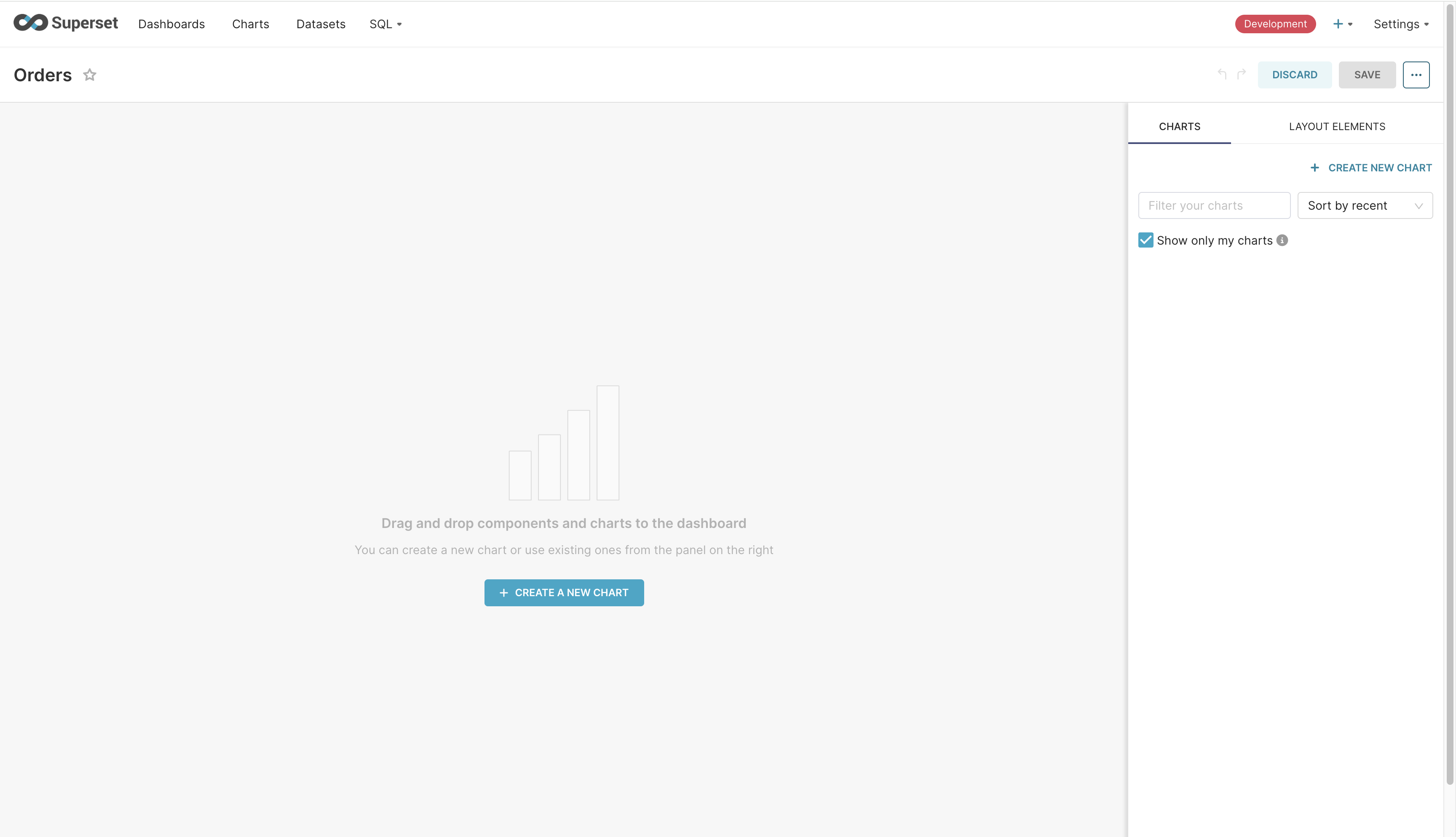
Click on “Dashboards” on the top-left and then click on “+ Dashboard”. This will create a new draft dashboard in which we’ll visualize datasets. Change its name to “Orders and click “Save”. You should see a screen similar to the one shown below.
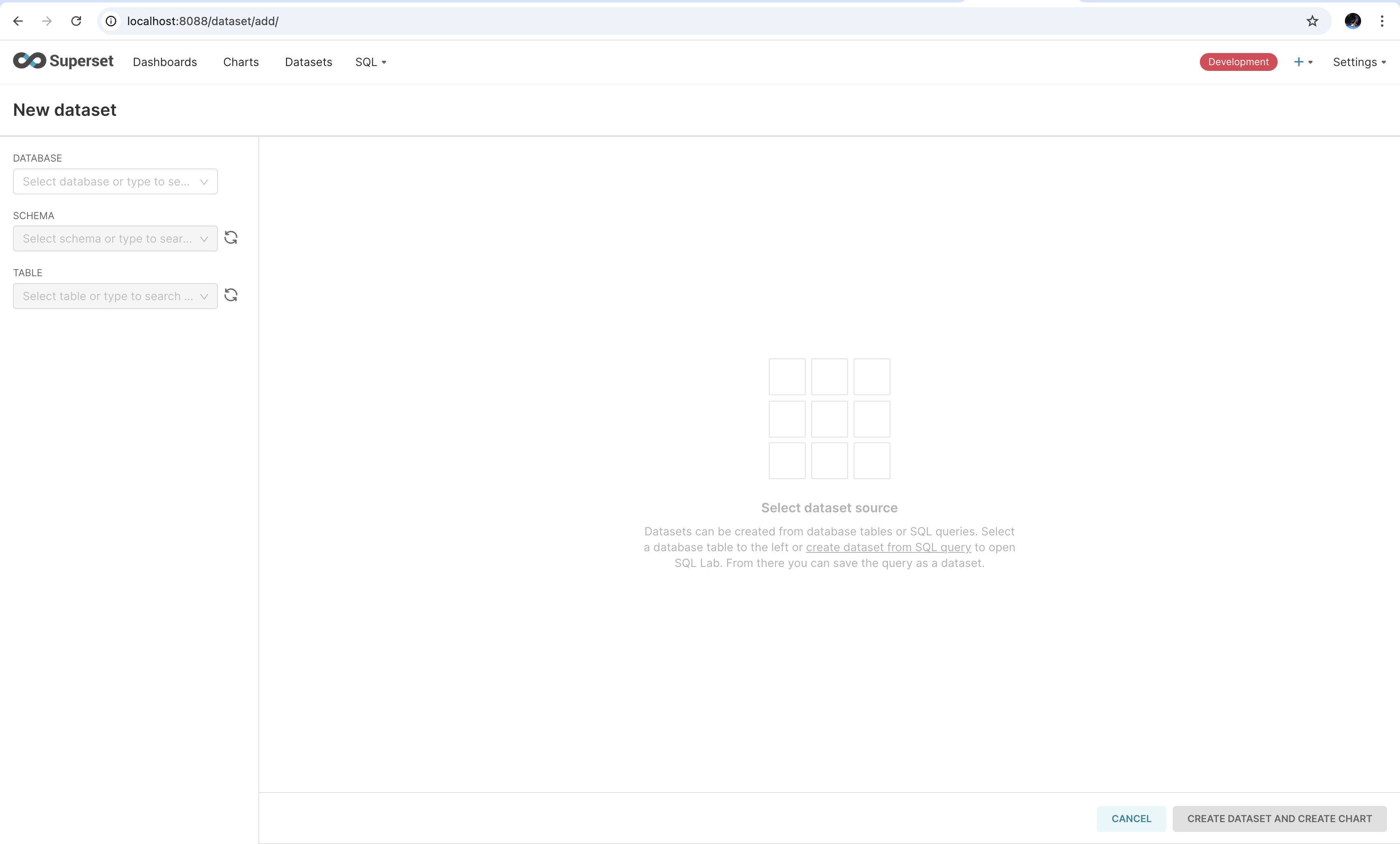
Click on “Create a new chart” button in the middle of the screen. From there, click on “Add a dataset”. Every chart needs to be associated with a dataset. We’ll create them based on the ones we’ve stored in Trino. You should see the following screen.
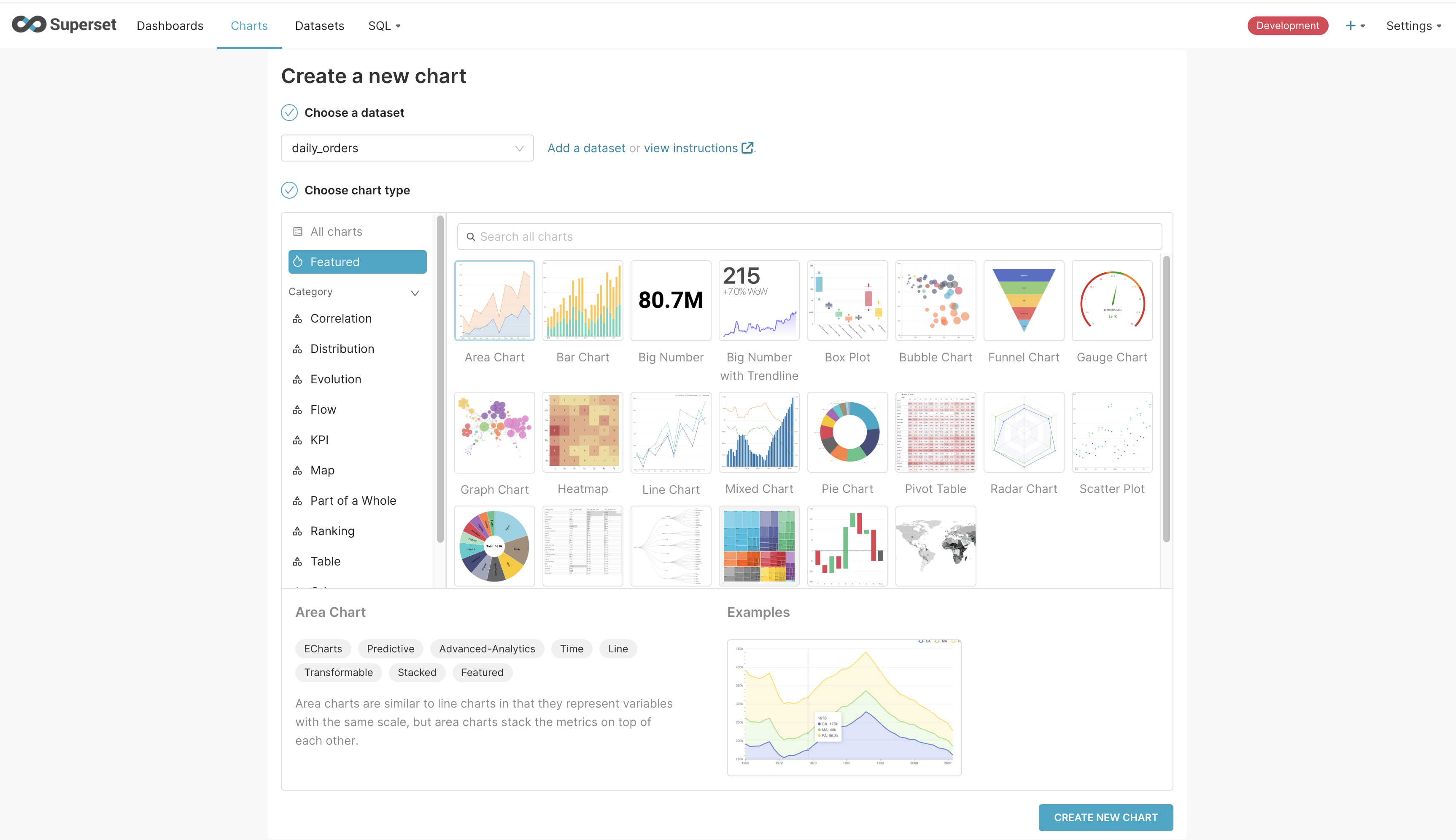
From the drop down on the left, select “Trino” as the database. Select the “views” schema. Finally, select “daily_orders” as the table. Once done, click on “Create Dataset and Create Chart” option on the bottom-right. In the screen that shows, select “Area Chart” and click on “Create New Chart”. This screen is shown below.
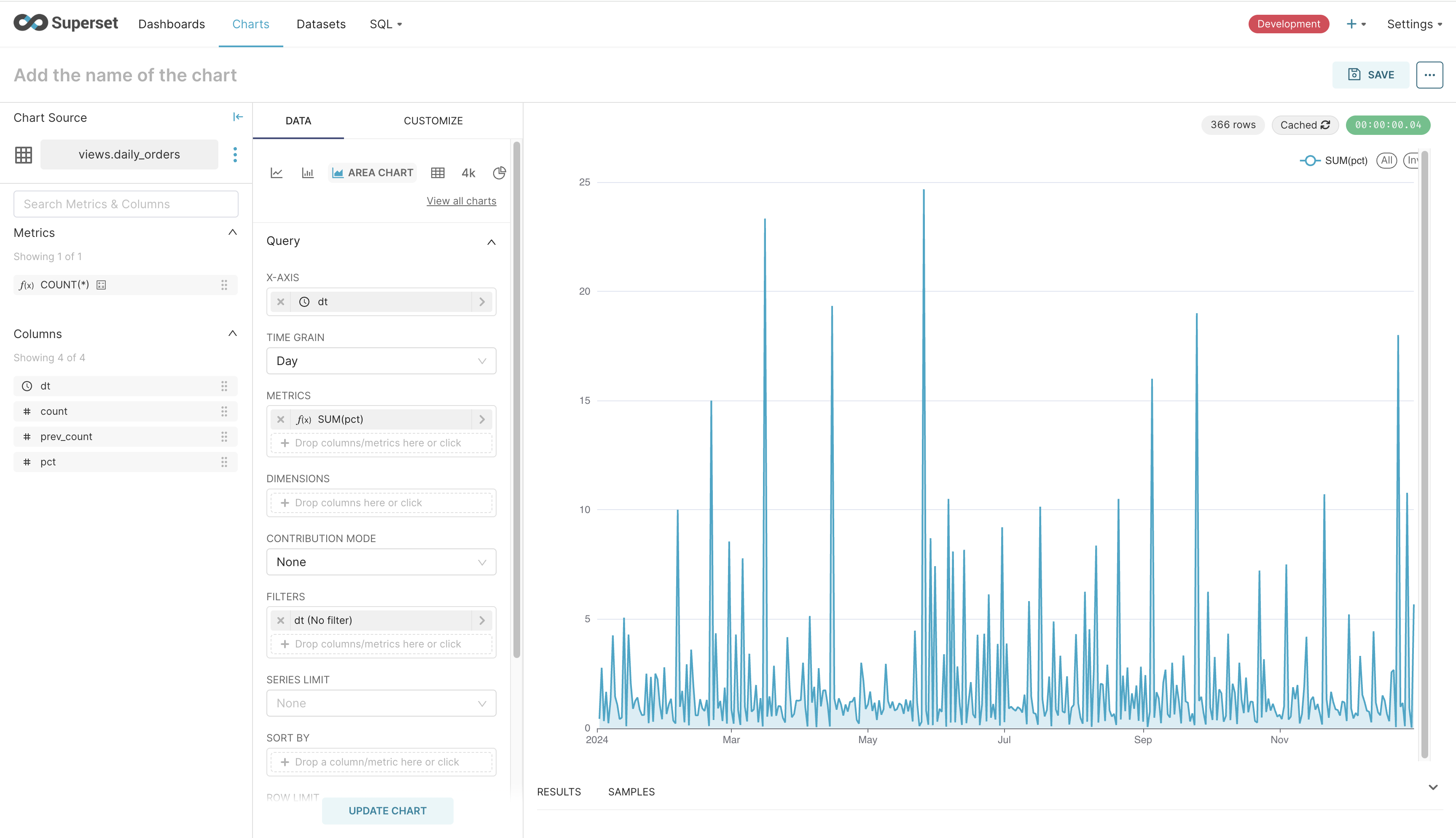
Once on the screen to create the chart, we’ll add the dt column to the X-axis and SUM(pct) to the Y-axis. Since there’s only one value for each day, SUM will return the same value. Clicking on “Update Chart” on the bottom causes a query to be fired to Trino and the result to be rendered as a line chart. It looks as follows.
Click on “Save” on the top-right. Give the chart a name and associate it with the dashboard we just created. It’ll take you to the dashboard with the chart rendered in it. Clicking on “Edit Dashboard” will allow you to change the size of the chart. Go ahead and increase its width. Saving the chart will make your dashboard look as follows.
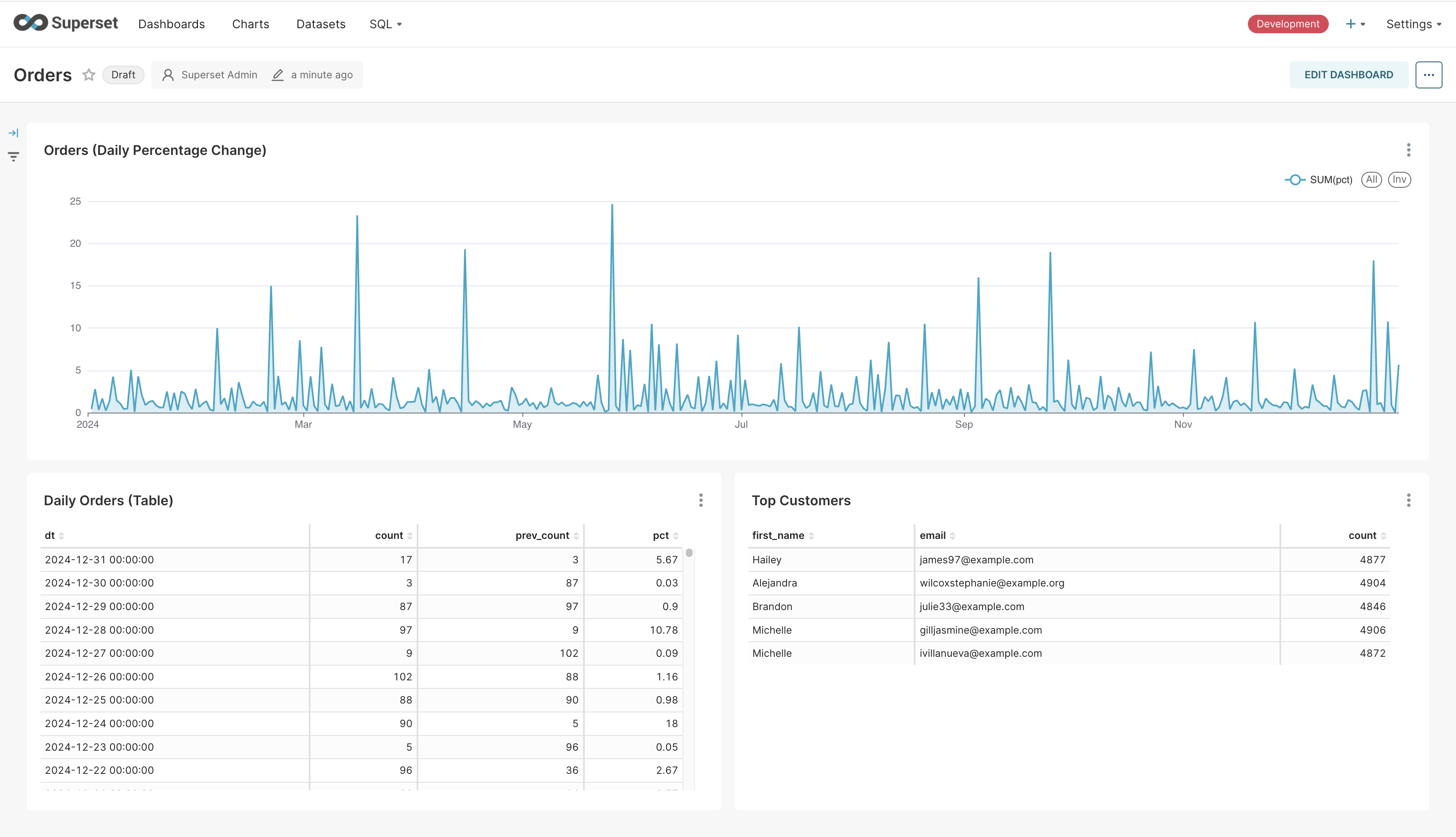
At this point, we can create more datasets and charts. I’ve created two more - one for displaying the data for the line chart as a table, and another for displaying the top customers. My final dashboard looks as follows.
The table and the line-chart are created from a view we’d created on top of Trino. Superset caches the results of the query for faster rendering. We can refresh the charts to see the latest data. Clicking on the three dots on the top-right of any chart will show the “Force refresh” option. Clicking on it will cause Superset to query Trino again to fetch the latest data. Since Pinot is getting updated in realtime and we have a view backing the chart, we’ll get the realtime numbers in the dashboard. We can make this happen automatically. Let’s go ahead and do that.
Click on “Edit dashboard”. Click on the three dots on the top-right and click on “Set auto-refresh interval”. In the pop-up that shows, select a frequency. Click “Save” to save this setting. Click “Save” one more time to save the dashboard. This will make the chart update in realtime without requiring the user to manually refersh it.
That’s it. That’s how you can create realtime dashbord on top of Pinot using Superset and Trino.
In the previous post we looked at how to query Pinot. We queried it using its REST API, the console, and Trino. In this post we’re going to look at how to use Apache Airflow to periodically create datasets on top of the data that’s been stored in Pinot. Creating datasets allows us to reference them in data visualization tools for quicker rendering. We’ll leverage Trino’s query federation to store the resultant dataset in S3 so that it can be queried using the Hive connector.
Getting started
Let’s say that the marketing team wants to run email campaigns where the users who actively place orders are given a promotional discount. The dataset they need contains the details of the user like their name and email so that the communication sent out can be personalised. We can write the following query in the source Postgres database to see what the dataset would look like.
1 2 3 4 5 6 7 8 9 10 11 12
SELECT u.id, u.first_name, u.email, COUNT(*) AS COUNT FROM public.user AS u INNERJOIN orders AS o ON u.id = o.user_id WHERE o.created_at >= NOW() -INTERVAL'30'DAY GROUPBY1, 2, 3 ORDERBY4DESC;
For us to create this dataset using Trino, we’ll have to ingest the user table into Pinot. Like we did in the earlier posts, we’ll use Debezium to stream the rows. We’ll skip repeating the steps here since we’ve already seen them. Instead, we’ll move to writing the query in Trino. Once we’ve written the query, we’ll look at how to use Airflow to run it periodically. I’ve also updated the orders table to extract the user_id column out of the source payload. Let’s translate the query written for Postgres to Trino.
1 2 3 4 5 6 7 8 9 10
SELECT u.id, u.first_name, u.email, COUNT(*) AS count FROM pinot.default.user AS u INNERJOIN pinot.default.orders AS o ON o.user_id = u.id WHERE FROM_UNIXTIME(CAST(o.created_at ASDOUBLE) /1e3) >= NOW() -INTERVAL'30'DAY GROUPBY1, 2, 3 ORDERBY4DESC;
We saw earlier that we’d like to save the result of this query so that the marketing team could use it. We can do that by storing the results in a table created using the above SELECT statement. Let’s create a schema in Hive called datasets where we’ll store the results. The following query creates the schema.
1 2 3 4
CREATE SCHEMA hive.datasets WITH ( "location" ='s3://apache-pinot-hive/datasets' );
We can now create the table using the above SELECT statement.
1 2 3 4 5 6 7 8 9 10
CREATETABLE hive.datasets.top_users AS SELECT u.id, u.first_name, u.email, COUNT(*) AS count FROM pinot.default.user AS u INNERJOIN pinot.default.orders AS o ON o.user_id = u.id WHERE FROM_UNIXTIME(CAST(o.created_at ASDOUBLE) /1e3) >= NOW() -INTERVAL'30'DAY GROUPBY1, 2, 3;
We can now query the table using the query that follows.
1 2
SELECT* FROM hive.datasets.top_users;
Having seen how to create datasets as tables using Trino CLI, let’s see how we can do the same using Airflow. Let’s say that the marketing team requires the data to be regenerated everyday. We can schedule an Airflow DAG to run daily to recreate this dataset. Briefly, Airflow is a task orchestrator. An orchestrator allows creating and executing workflows expressed as directed acyclic graphs (DAGs). Each workflow consists of multiple tasks, which form the nodes in the graph, and edges between the tasks indicate the directionality.
We’ll create a workflow which recreates the dataset daily. In a nutshell, the workflow first drops the older table and then recreates a newer one. This is because the Trino connector does not allow creating or replacing table as an atomic operation. We’ll leverage Airflow’s SQL operator and templating mechanism to create and execute queries. The following shows the files and folders we’ll be working with as we create the DAG.
1 2 3 4 5 6 7 8 9
$ tree airflow/dags airflow/dags ├── __init__.py ├── create_top_users_dataset.py └── sql ├── common │ ├── drop_table.sql └── datasets └── top_users.sql
Let’s begin with the drop_table.sql query. This is a templated query which allows dropping a table. Writing queries as templates allows us to leverage the Jinja2 templating engine that comes with Airflow. We can create queries depending on the parameters passed to the operator. This allows reusing the same template across multiple tasks. The variables are enclosed in two pairs of braces and the name of the variable is written between them. The content of the file is shown below.
1
DROP TABLE IF EXISTS {{ params.name }}
As we’ll see shortly, we’ll pass parameters to the Airflow task executing this query which are available in the params dictionary in the template. In the query above, we’d have to pass the name variable which contains the name of the table we’d like to drop. The top_users.sql file contains the same query we’ve seen above so we’ll move on to setting up the DAG.
The DAG is written in the file create_top_users_dataset.py and contains two tasks. First, to drop the table, which uses the templated query above. Second, to create the dataset. Both of these tasks use the SQLExecuteQueryOperator. Its parameters include a connection ID, which is used to connect to the database, the path to the SQL file containing the templated query to execute, and the values for the parameters. The contents of the file are shown below.
# -- Dependencies between tasks drop_table >> create_table
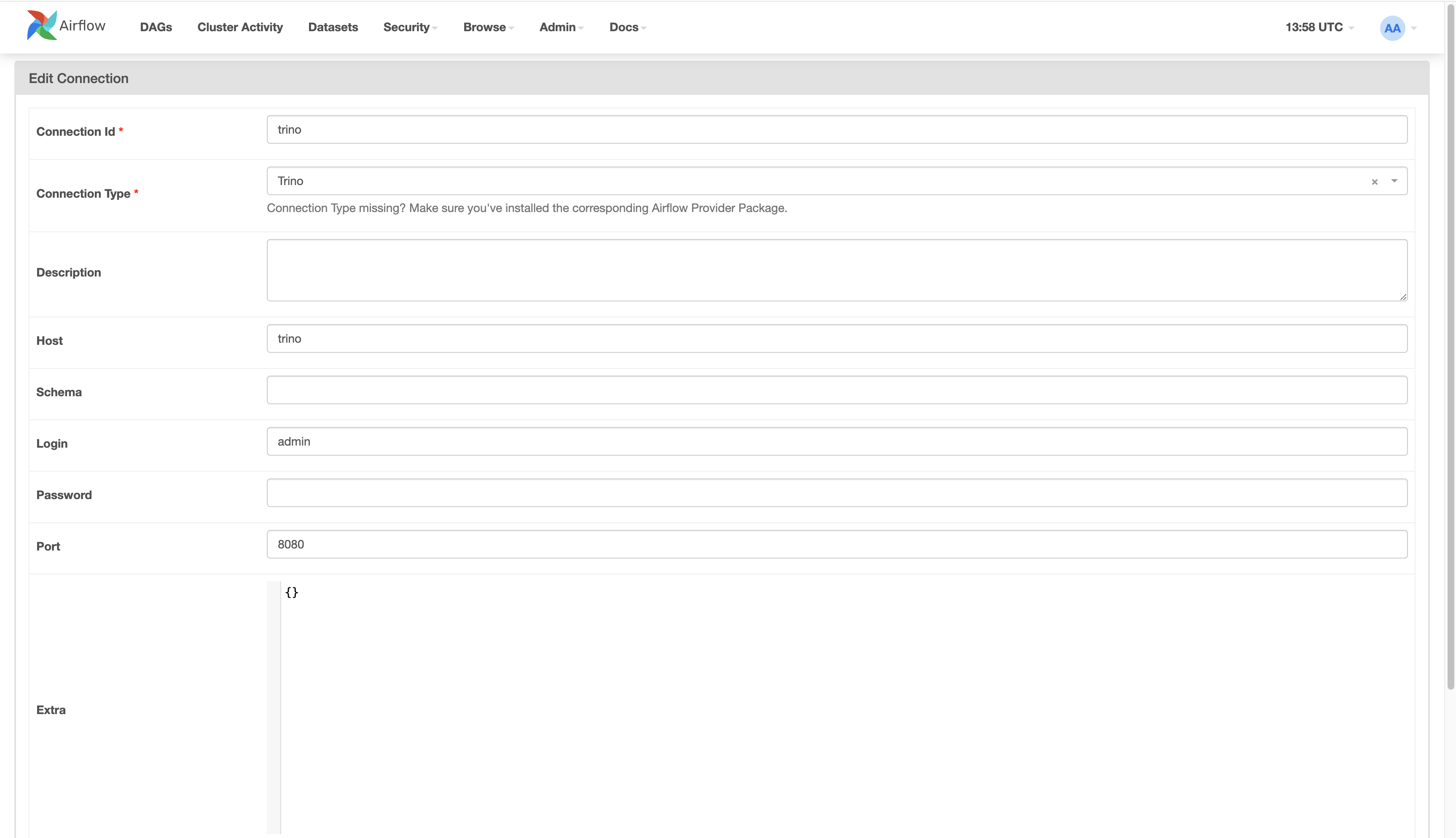
We define the DAG in line 6 and specify that it will execute daily. Line 13 and 21 define the tasks within the DAG. The first task drops the table, if it exists. The second task creates the table again. On line 29 we define the relationship between the tasks. Both of the tasks are of type SQLExecuteQueryOperator. This task allows executing arbitrary SQL queries by connecting to a database. The connection to the database is specified as the conn_id; we’ve specified it as trino. As we’ll see next, we need to create the connection using the Airflow console. Once we create the connection, we can execute the DAG.
Airflow UI is available on http://localhost:8080. From there we’ll click on ‘Admin’ up top, and then ‘Connections’. From there we’ll click on the ‘+’ icon to create a connection. The screenshot below shows what we need to fill in to make the connection. In my setup, Trino runs with the hostname trino and you’ll have to replace this to match what you have. Once the details are entered, we’ll click the ‘Save’ button at the bottom to create the connection.
Finally, we can trigger the DAG. We’ll click on the ‘DAGs’ option on top left side of the screen. This will show us the list of DAGs available. From there, we’ll click the play button for the create_daily_datsets DAG. This will trigger and run the DAG. We’ll wait for the DAG to finish running. Assuming everything works correctly, we will have created a table in S3. Leaving the DAG in the enabled state causes it to run on the specified schedule; in this case it is daily. As the DAG continues to run, it’ll create and recreate the table daily.
That’s it on orchestrating tasks to create datasets on top of Pinot.
In the previous post we looked at nullability and how Pinot requires that a default value be specified in place of an actual null. In this post we’ll begin looking at how to query data stored in Pinot. We’ll begin by querying Pinot using its API and query console. Then, we’ll query Pinot using Trino. We’ll use Trino’s query federation capability to create views and tables on top of the data that’s stored in Pinot.
Getting started
Pinot provides an SQL interface for writing queries that’s built on top of the Apache Calcite query parser. It ships with two query engines - the single-stage engine called v1 and the multi-stage engine called v2. The single-stage engine allows writing simpler SQL queries that do not involve joins or window functions. The multi-stage query engine allows more complex queries involving joins on distributed tables, window functions, common table expressions, and much more. It’s optimized for in-memory processing latency. Queries can be submitted to Pinot using the query console, REST API, or Trino. When querying Pinot using either the API or query console, we need to explicitly enable the multi-stage engine.
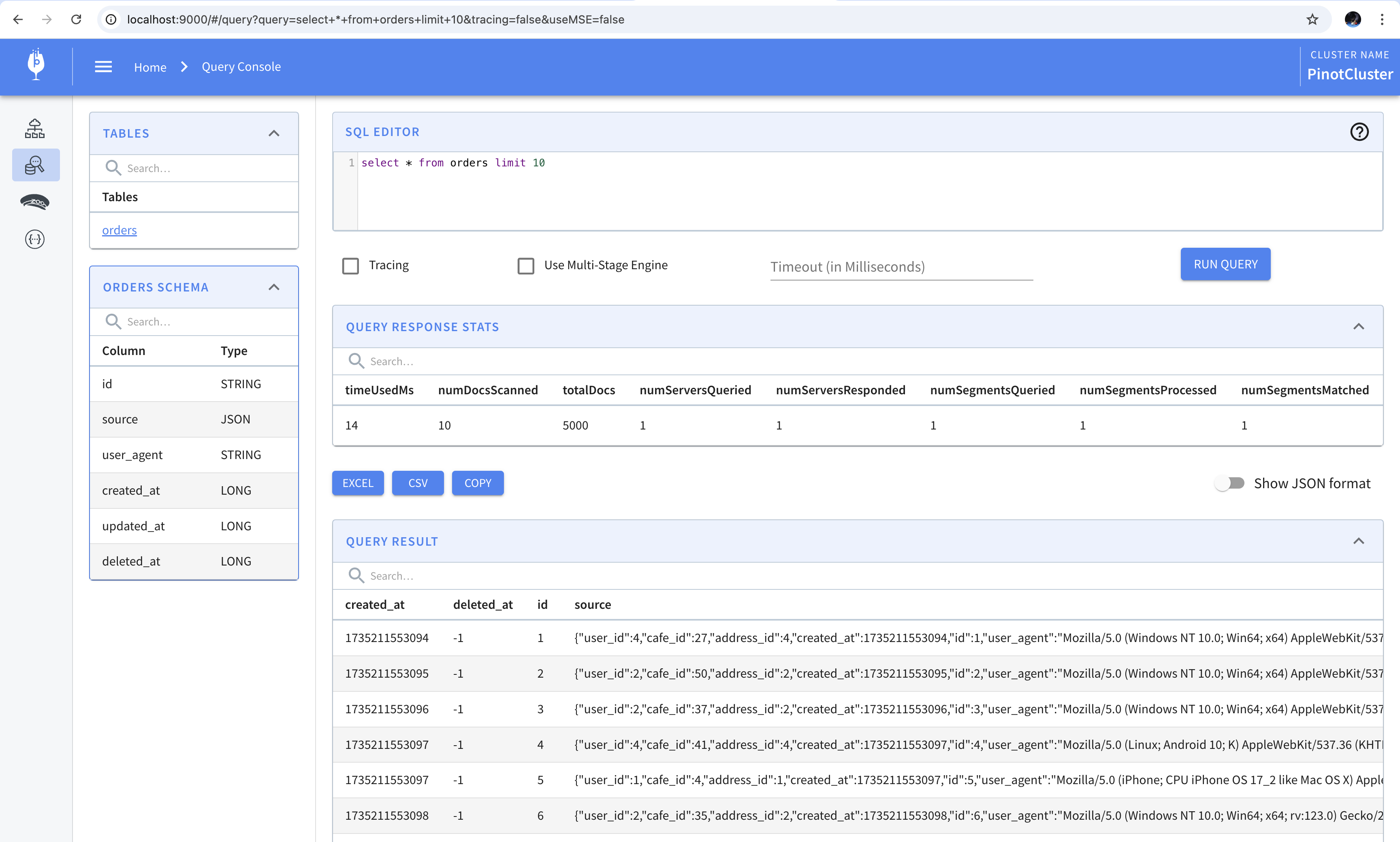
We’ll begin by writing SQL queries and submitting them first using the API and then using the query console. For queries that require a lot of data shuffling or data that spills to disk, it is recommended to use Presto or Trino. Let’s start by writing a simple SQL query that retrieves the user agent from the orders table. The SQL query to do this is given below.
1
SELECT user_agent FROM orders LIMIT 1;
We’ll create a file called query.json which contains the payload that we’ll POST to Pinot. It contains the SQL query and options to indicate to Pinot that we’d like to use the multi-stage engine to execute the query. The content of the file is given below.
1 2 3 4 5
{ "sql":"SELECT user_agent FROM orders LIMIT 1;", "trace":false, "queryOptions":"useMultistageEngine=true" }
We can now POST this payload to the appropriate endpoint using curl.
The response is returned as a large JSON object but the part we’re interested in is stored in the key called resultTable. It contains the names of the columns returned, the values of the columns, and their datatypes. The following shows the result returned for the query that we’ve submitted above.
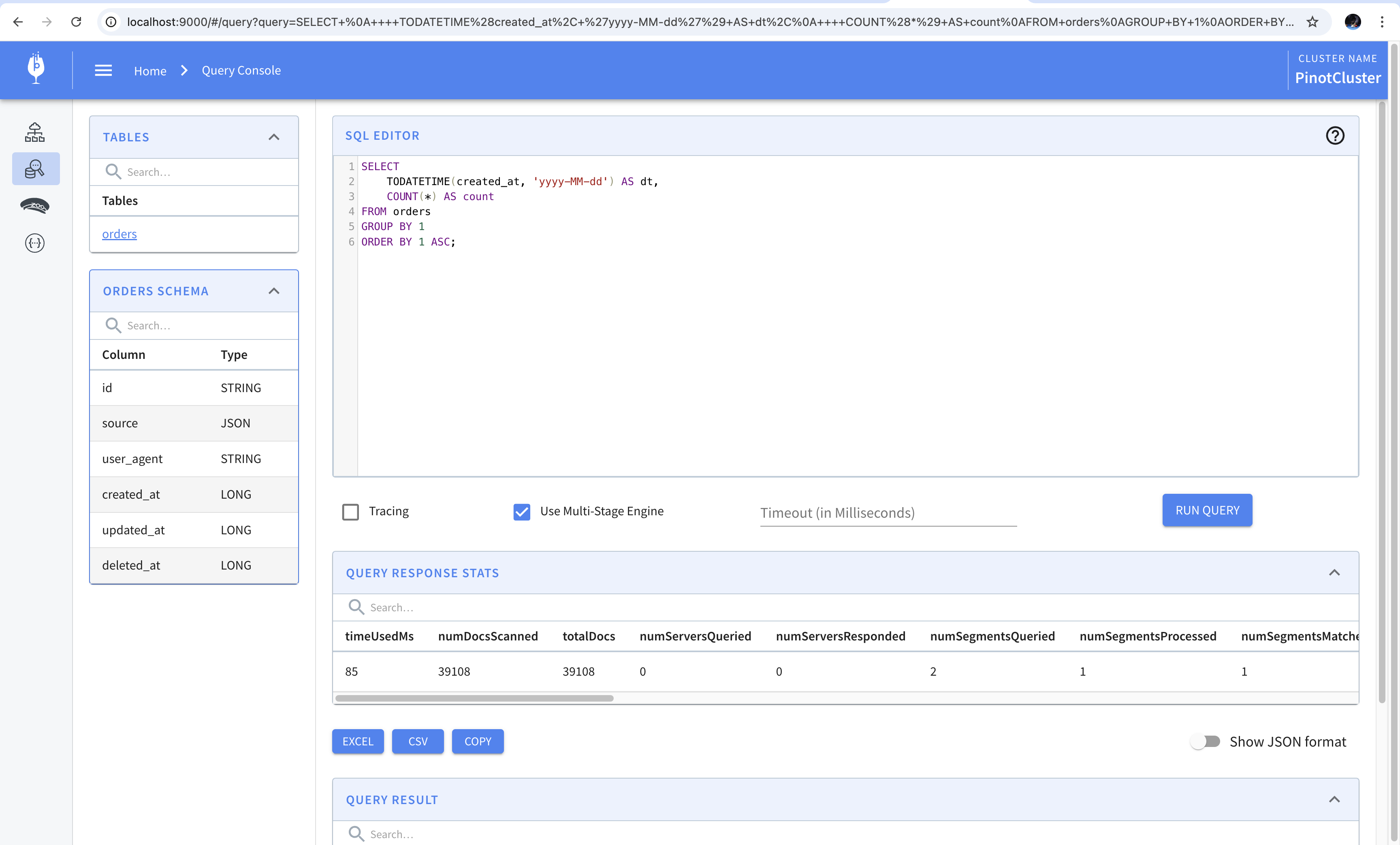
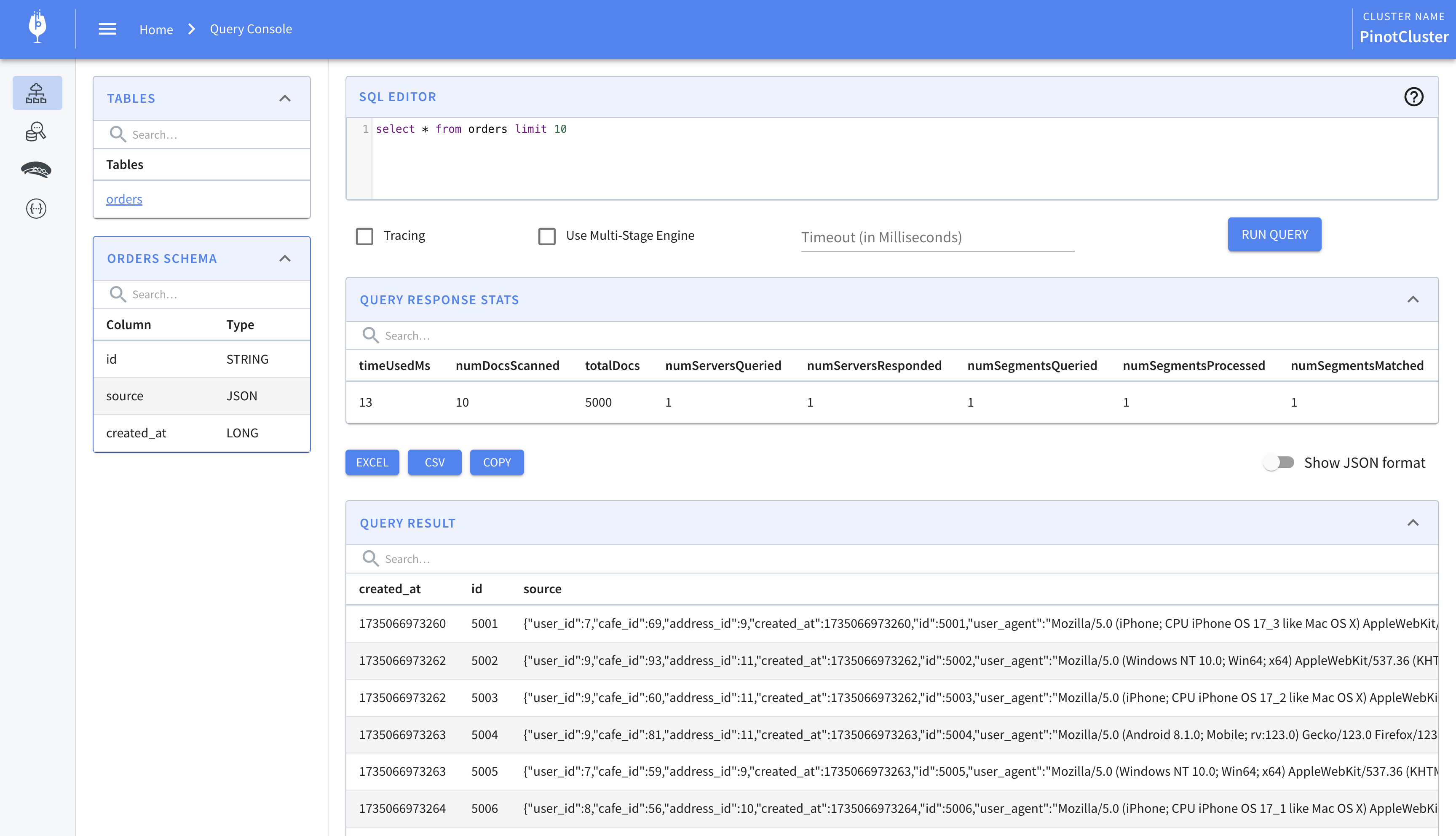
We’ll now look at writing SQL queries using the query console. Let’s write a SQL query which counts the number of orders placed each day. To do this, we’d have to convert the created_at column from milliseconds to date and then run a group by to find the count of the orders that have been placed. The following query gives us the desired result.
1 2 3 4 5 6
SELECT TODATETIME(created_at, 'yyyy-MM-dd') AS dt, COUNT(*) AS count FROM orders GROUPBY1 ORDERBY1ASC;
We can run this in the console using the single-stage engine since it is one of the simpler queries. To do this, we’ll paste the query in the query console and leave the “Use Multi-Stage Engine” checkbox unchecked. The result of running the query is shown in the screenshot below.
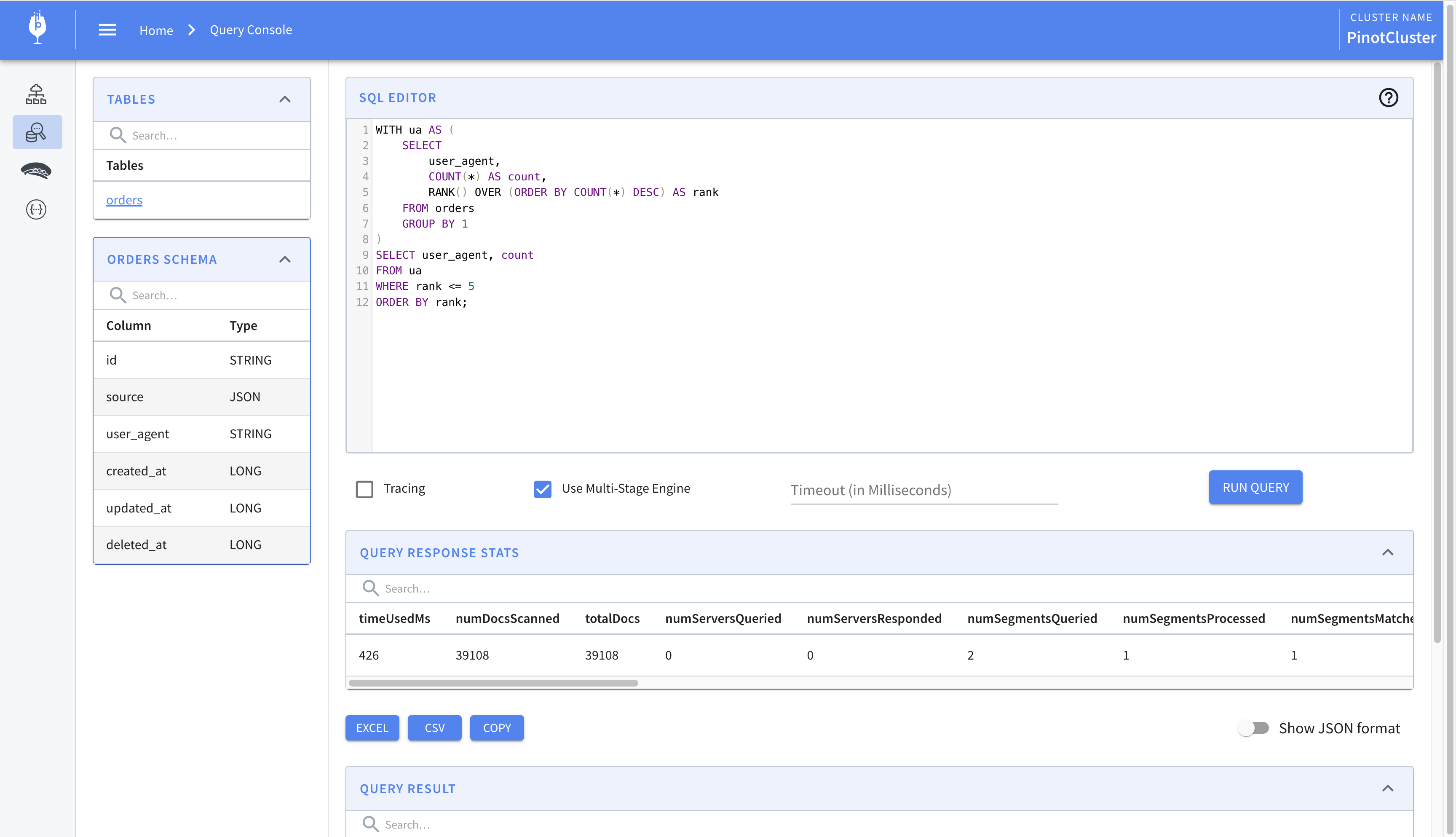
We’ll now modify the query so that it requires the multi-stage engine. Using features of SQL language like window functions, common table expressions, joins, etc. requires executing the query using the multi-stage engine. We’ll write a query which finds the top five user agents and ranks them. This requires using common table expressions, and window functions and is the perfect candidate for using the multi-stage engine. The query is shown below.
1 2 3 4 5 6 7 8 9 10 11 12
WITH ua AS ( SELECT user_agent, COUNT(*) AS count, RANK() OVER (ORDERBYCOUNT(*) DESC) AS rank FROM orders GROUPBY1 ) SELECT user_agent, count FROM ua WHERE rank <=5 ORDERBY rank;
The result of running this query is shown below. Notice how the checkbox to use the multi-stage engine is checked.
Having seen how to query Pinot using the API, and the query console with either single-stage or multi-stage engine, we’ll move on to querying Pinot using Trino. We’ll begin by connecting to Trino using its CLI utility and create a catalog which connects to our Pinot instance. Then, we’ll run queries using Trino. We’ll also see how we can leverage query federation provided by Trino to connect to AWS Glue and create views and tables on top of the data stored in Pinot.
Let’s start by connecting to Trino. The following command shows how to connect to the Trino instance running as a Docker container using its command-line utility. You can follow the instructions mentioned in the official documentation to setup the CLI.
1
./trino http://localhost:9080
Every database in Trino that we’d like to connect to is configured using a catalog. A catalog is a collection of properties that specify how to connect to the database. We’ll begin by creating a catalog which allows us to query Pinot.
1 2 3 4
CREATE CATALOG pinot USING pinot WITH ( "pinot.controller-urls" = 'pinot-controller:9000' );
The CREATE CATALOG command creates a catalog. It takes the name of the catalog, which we’ve specified as pinot, and the name of the connector which connects to the database, which we’ve also specified as pinot. The WITH section specifies properties that are required to connect to the database. We’ve specified the URL of the controller. Once the catalog is created, we can begin querying the tables in the database. The tables in Pinot are stored in the default schema of the pinot connector. To be able to query these, we’ll have to USE the catalog and schema. The following command sets the schema for the current session.
1
USE pinot.default;
To view the tables in the current schema, we’ll execute the SHOW TABLES command.
Let’s build upon the query that we wrote previously which calculates the count of the orders placed on a given day. Let’s say we’d like to find the percentage change between the number of orders placed on a given day and the day prior. We can do this using the LAG window function which will allow us to access the value of the prior row. The following query shows how to calculates this.
1
2
3
4
5
6
7
8
9
10
11
12
13
14
WITHFUNCTION div(x DOUBLE, y DOUBLE) RETURNSDOUBLE RETURN x / y WITH ua AS ( SELECTCAST(FROM_UNIXTIME(created_at /1e3) ASDATE) AS dt, COUNT(*) AS count FROM orders GROUPBY1 ) SELECT dt, count, LAG(count, 1) OVER (ORDERBY dt ASC) AS prev_count, ROUND(DIV(count, LAG(count, 1) OVER (ORDERBY dt ASC)), 2) AS pct FROM ua;
There’s a lot going on in the query above so let’s break it down. We begin by defining an inline function called DIV which performs division on two numbers. The reason for writing this function is that the division operator in Pinot returns the integer part of the quotient. To get the quotient as a decimal, we’d have to cast the values to DOUBLE. The function does just that. In the common table expression, we calculate the number of orders placed each day. Finally, in the SELECT statement, we find the number of orders placed on the day prior using the LAG window function.
Let’s now say that we’d like to run the query frequently. Perhaps we’d like to display the table in a visualization tool. One way to do this would be to store the query as a view. However, Pinot does not support views. We’d have to work around this by relying on Trino’s query federation to write the result to another data store which supports creating views. For the sake of this post, we’ll use AWS Glue as a replacement for HDFS.
Let’s start with creating a Hive catalog in which we use S3 as the backing store.
In the query above, we’re creating the Hive catalog which we’ll use to create and store datasets. Since we’re storing files in S3, we need to specify the region and its S3 endpoint. You’d have to replace the keys with those of your own if you’re running the example locally.
Once we create the catalog, we’ll have to create the schema where datasets will be stored. Schemas are created with CREATE SCHEMA command and require that we provide a path in an S3 bucket where the files will be stored. The query below shows how to create a schema named views.
1 2 3 4
CREATE SCHEMA hive.views WITH ( "location" = 's3://apache-pinot-hive/views' );
Once the schema is created, we can persist the query or its results for quicker access. In the query that follows, we create a view on top of Pinot.
1 2 3 4 5 6 7 8 9 10 11 12
CREATEVIEW hive.views.daily_orders AS WITH ua AS ( SELECTCAST(FROM_UNIXTIME(created_at /CAST(1e3ASDOUBLE)) ASDATE) AS dt, COUNT(*) AS count FROM pinot.default.orders GROUPBY1 ) SELECT dt, count, LAG(count, 1) OVER (ORDERBY dt ASC) AS prev_count, ROUND(CAST(count ASDOUBLE) /LAG(count, 1) OVER (ORDERBY dt ASC), 2) AS pct FROM ua;
We can query the view once it is created. This allows us to save the queries so that they can be referenced in data visualization tools. In the view above, we’ll get the realtime difference between orders placed since Pinot will be queried every time we select from the view. A small caveat to note is that views cannot store inline functions so we had to cast one of the operands in the division operation to double manually.
To see this in action, we’ll run the data generation script one more time and then query the view. We can see that the counts for orders placed today, yesterday, and day before yesterday increase after the script runs.
Creating views like this provides us with a way to save queries that we’d like to run frequently. As we’ll see in later posts, these can also be referenced in data visualization tools to provide realtime analytics.
In the previous post we looked at evolving the schema. We briefly discussed handling null values in columns when we added the user_agent column. It allows null values since enableColumnBasedNullHandling is set to true. However, we weren’t able to see nullability in action since that column always had values in it. In this post we’ll evolve the schema one more time and add columns that have null values in them. We’ll see how to handle null values in Pinot queries, and how they differ from nulls in other databases. Let’s dive right in.
Getting started
We’ll begin by looking at the source payload that we’ve stored in Pinot.
In the payload above, we notice that there’s created_at but no updated_at or deleted_at. That’s because these have null values in the source table in Postgres. Let’s update the schema and table definitions to store these fields.
To update the schema, we’ll add the following to dateTimeFieldSpecs.
In the JSON above, we specify the usual fields just as we did for created_at. We also set defaultNullValue. This value will be used instead of null when these fields are extracted from the source payload. This is different from what you’d usually observe in a database that supports null values. The reason for this is that Pinot uses a forward index to store the values of each column. This index does not support storing null values and instead requires that a value be provided which will be stored in place of null. In our case, we’ve specified -1. The value that we specify as a default must be of the same data type as the the column. Since the two fields are of type LONG, specifying -1 suffices.
We’ll PUT this schema using the following curl command.
Now when we open the query console, we’ll see the table with updated_at and deleted_at fields with their values set to -1.
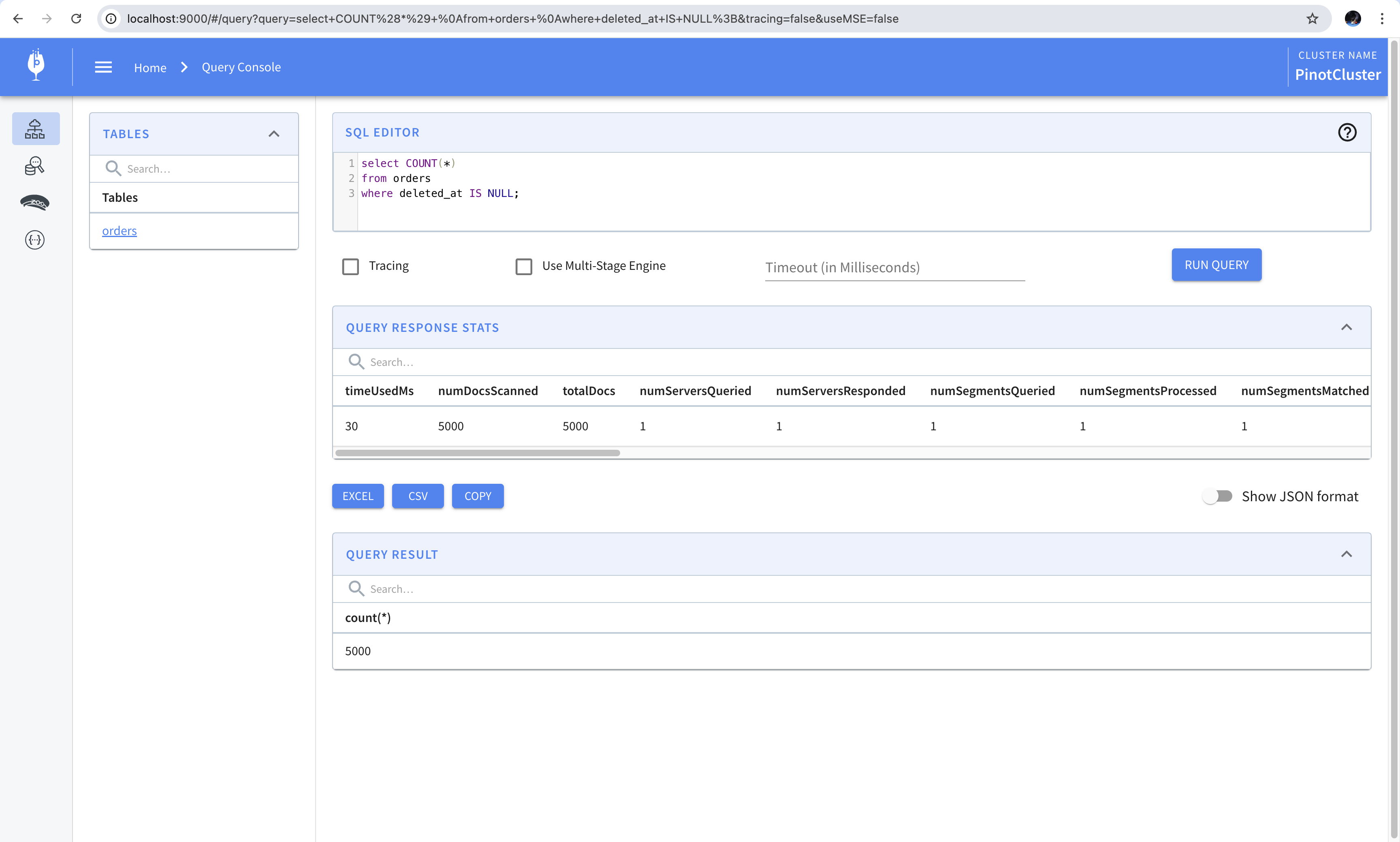
We know that we have a total of 5000 rows where the deleted_at field is set to null. This can be verified by running a count query in Pinot. This shows that although the values in the column are set to -1, Pinot identifies them as null and returns the correct result.
1 2 3
SELECTCOUNT(*) FROM orders WHERE deleted_at ISNULL;
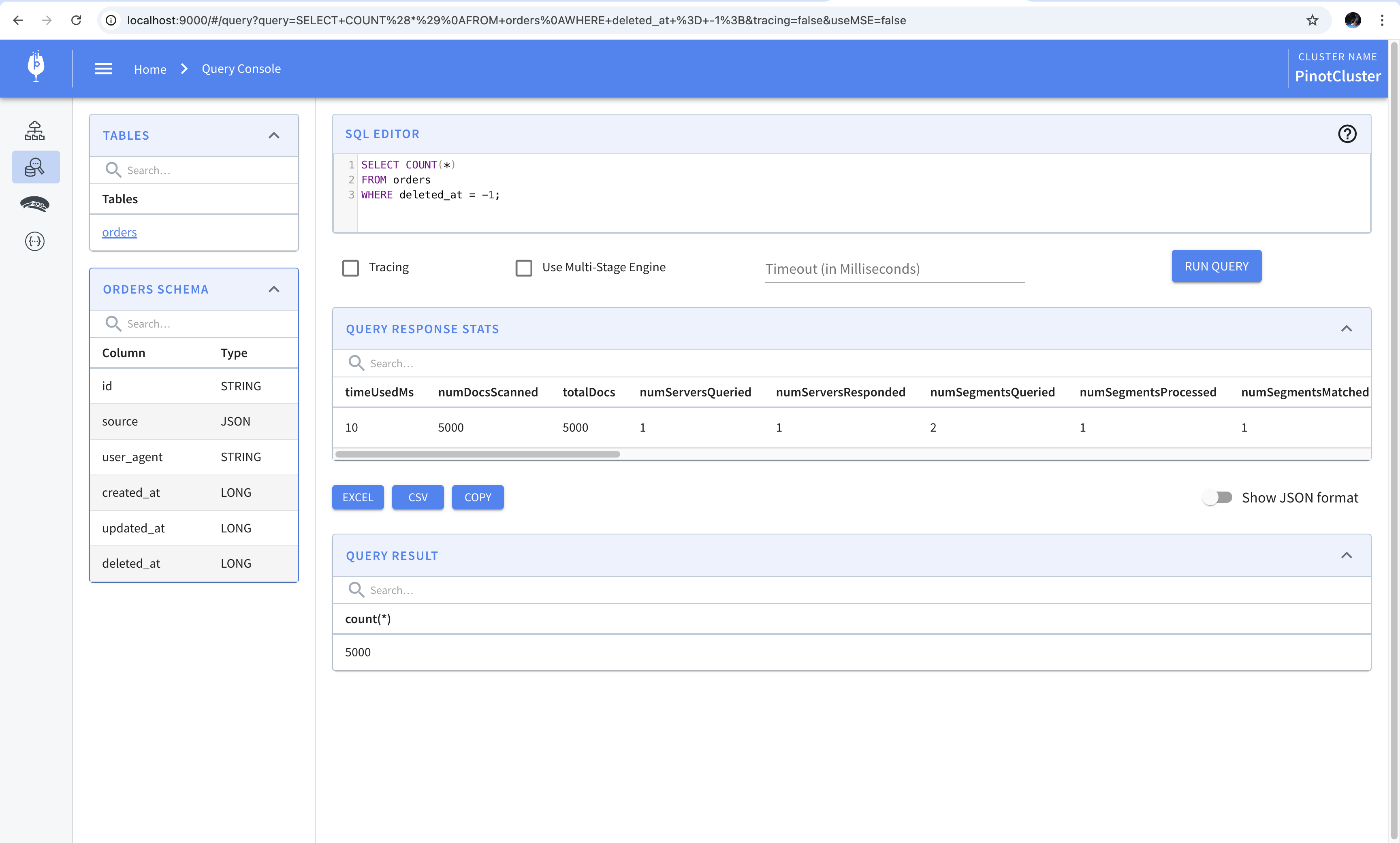
A workaround suggested in the documentation is to use comparison operators to compare against the value used in place of null. For example, the following query will produce the same result as the one shown above.
In the previous post we saw how to ingest the data into Pinot using Debezium. In this post we’re going to see how to evolve the schema of the tables stored in Pinot. We’ll begin with a simple query which computes an aggregate on the user agent column stored within the source payload. Then, we’ll extract the value of user agent column out of the source payload into a column of its own.
Getting started
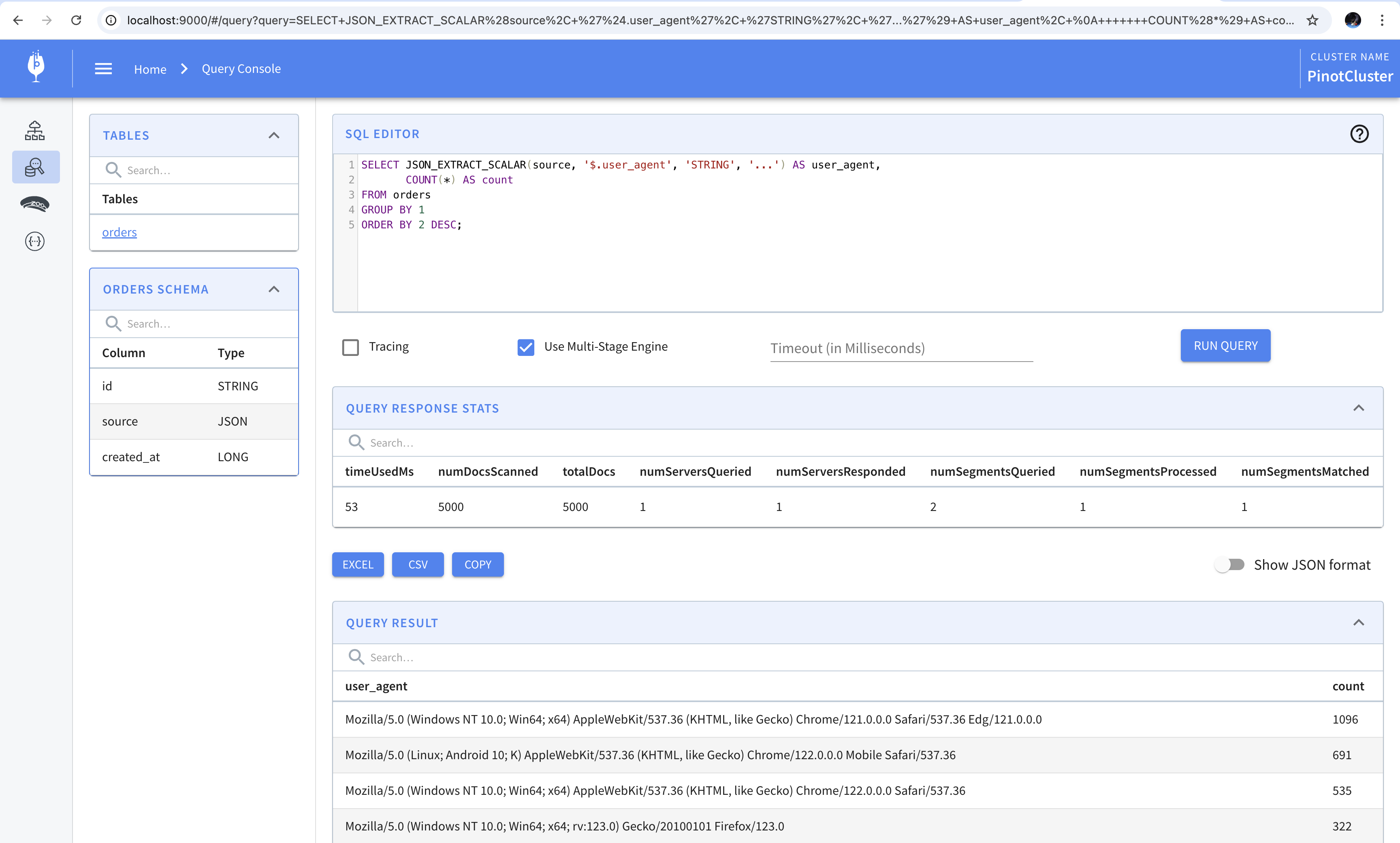
Let’s start with a simple query. Let’s count the number of times each user agent appears in the table and sort it in descending order. We can do this using the following SQL query.
1 2 3 4 5
SELECT JSON_EXTRACT_SCALAR(source, '$.user_agent', 'STRING', '...') AS user_agent, COUNT(*) AS count FROM orders GROUPBY1 ORDERBY2DESC;
The result of running this query is shown below.
Let’s take a closer look at the query. To extract values out of the source column, we use the JSON_EXTRACT_SCALAR() function. It takes the name of the column containing the JSON payload, the path of the value within the payload, the datatype of the value returned, and the value to be used as a replacement for null.
For a simple query like this, using JSON_EXTRACT_SCALAR() works. However, it becomes unwieldy when there are more than one column to extract or when writing ad-hoc business analytics queries that join multiple tables on values present within a JSON column. Writing SQL would be easier if we could extract the value out of the JSON payload into a column of its own.
To extract the values out of the source payload into its own column, we’ll have to update the schema and table definitions. We’ll update the schema definition to add new columns, and we’ll update the table definition to extract fields out of the source column using field-level transformations.
We’ve added user_agent as a new column under dimensionFieldSpecs. Notice that we’ve set enableColumnBasedNullHandling to true. This allows columns to store null values in them. In Pinot, allowing or disallowing null values is configured per-table. The recommended way is to use column-based null handling where each column is configured to allow or disallow null values. This is what we’ve used in our schema above. The id, source, and created_at columns do not allow null values in them since they have notNull set to true. The user_agent column allows null values in it since it is implicitly nullable.
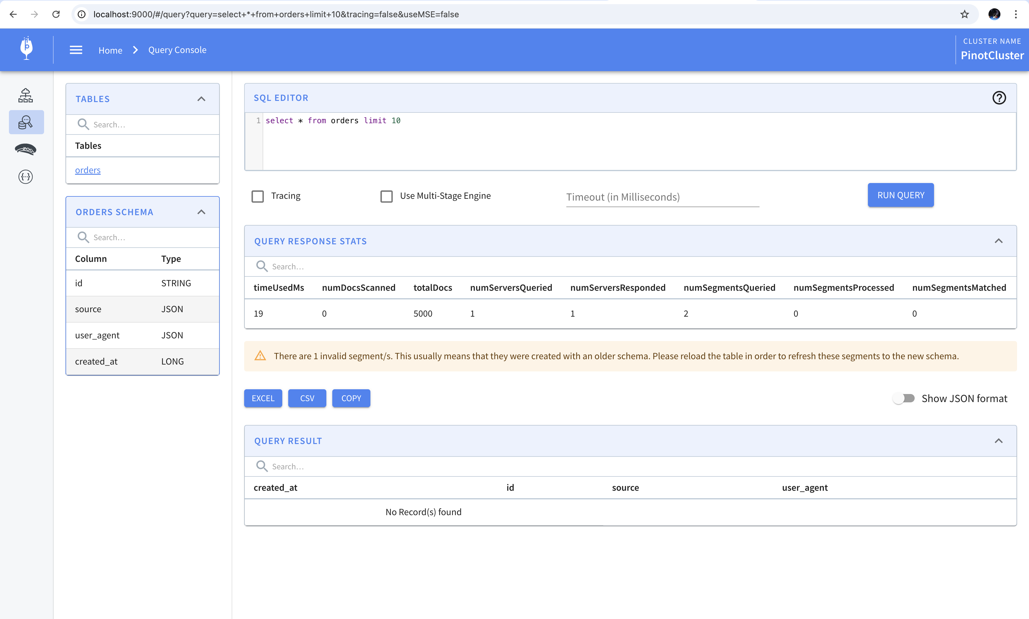
Upon opening the query console we find that there’s an error message. This message indicates that the segments are invalid because they were created using an older version of the schema. We can reload all the segments to fix this error but we’ll get to that in a minute. We’ll first update the table definition.
To update the table definition, we’ll add the following field-level transformation to the transformConfigs.
In this transformation we’re extracting the user_agent field into a column with the same name. Notice how we’re referencing the source column instead of the payload emitted by Debezium to get the value. Once we’ve made this change we’ll PUT the new table definition using curl.
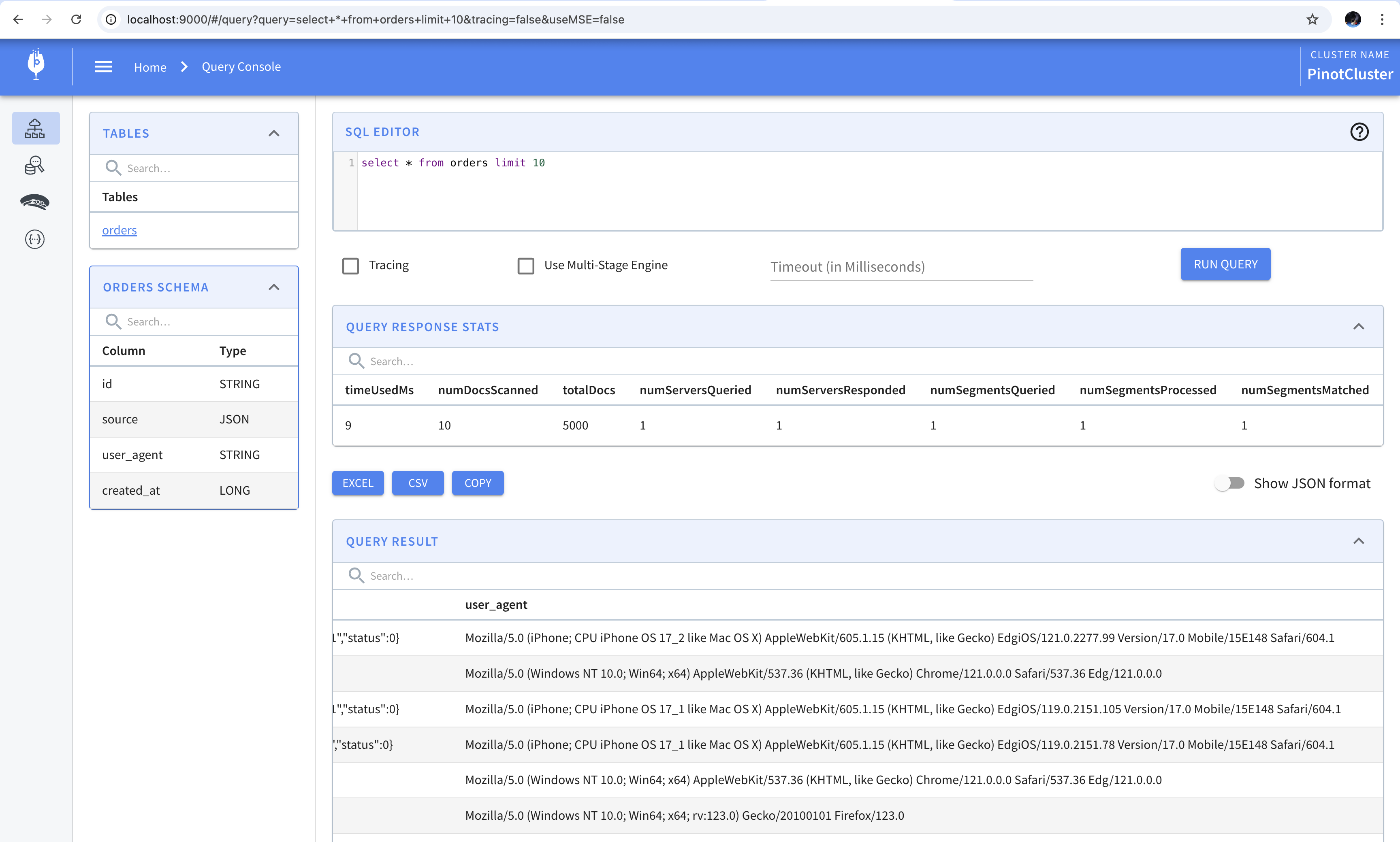
Upon opening the query console, we find that the a new user_agent column has been added to the table.
It’s common for the table to change with time as new columns are added. Consequently, the schema and table definitions will evolve in Pinot. As we update the schema in Pinot, we have to keep in mind that columns can only be added and not removed. In other words, the schema needs to remain backwards compatible. If you’d like to drop a column or rename it, you’ll have to recreate the table.
In the first part we saw the overall design of the system. In the second part we created a dataset that we can work with. In this post we’ll look at the first category of components and these are the ones that bring the data into the platform. We’ll see how we can stream data from the database using Debezium and store it in Pinot realtime tables.
Before we begin
The setup is still Dockerized and now has containers for Debezium, Kafka, and Pinot. In a nutshell, we’ll stream data from the Postgres instance into Kafka using Debezium and then write it to Pinot tables.
Getting started
In the first part of the series we briefly looked at Debezium. To recap, Debezium is a platform for change data capture. It consists of connectors which capture change data from the database and emit them as events into Kafka. Which database tables to monitor and which Kafka topic to write them to are specified as a part of the connector’s configuration. This configuration is written as a JSON object and sent to a specfic endpoint to spawn a new connector.
We’ll begin by creating configuration for a connector which will monitor all the tables in the database and route each of them to a dedicated Kafka topic.
There are two main parts to this configuration - name and config. The name is the name we’ve given to the connector. The config contains the actual configuration of the connector. We specify quite a few things in the config object. We specify the class of the connector which is the fully qualified name of the Java class, the credentials to connect to the database, whether or not to take a snapshot, how to route the data to the appropriate Kafka topics, and how to pass signals to Debezium.
While most of the configuration is self-explanatory, we’ll look closely at the ones related to snapshot, signalling, and routing. We set the snapshot mode to no_data which means that the connector will stream historical rows from the database. The only rows that will be emitted are the ones created or updated after the connector began running. We’ll use this setting in conjunction with signals to incrementally snapshot the tables we’re interested in. Signals are a way to modify the behavior of the connector, or to trigger a one-time action like taking an ad-hoc snapshot. When we combine no_data with signals, we can tell Debezium to selectively snapshot the tables we’re interested in. The signal.data.collection property specifies the name of the table which the connector will monitor for any signals that are sent to it.
Finally, we specify a route transform. We do this by writing a regex which matches against the fully qualified name of the table, and extracts only the table name. This allows us to send the data from every table into a dedicated Kafka topic of its own.
Notice how we’ve not specified which tables to monitor. Since it is a Postgres database, the connector will monitor all the tables in all the schemas within the database and stream them. Now that the configuration is created, we’ll POST it to the appropriate endpoint to create the connector.
Now that the connector is created, we will signal it to initiate a snapshot. Signals are sent to the connector using rows inserted into the table. We’ll execute the following INSERT query to tell the connector to take a snapshot of the orders table.
The row tells the connector to initiate a snapshot, as indicated by execute-snapshot, and stream historical rows from the orders table in all the schemas within the database. It is an incremental snapshot so it will happen in batches. If we docker exec into the Kafka container and use the console consumer, we’ll find that all the rows eventually get streamed to the topic. The command to show it is given below.
1
2
[kafka@kafka ~]$ kafka-console-consumer.sh --bootstrap-server kafka:9092 --topic orders --from-beginning | wc -l
^CProcessed a total of 5000 messages
We can compare this with the row count in the table using the following SQL command.
Now that the data is in Kafka, we’ll move on to how to stream it into a Pinot table. Before we get to that, we’ll look at what a table and schema are in Pinot.
A table in Pinot is similar to a table in a relational database. It has rows and columns where each column has a datatype. Tables are where data is stored in Pinot. Every table in Pinot has an associated schema and it is in the schema where the columns and their datatypes are defined. Tables can be realtime, where they store data from a streaming source such as Kafka. They can be offline, where they load data from batch sources. Or they can be hybrid, where they load data from both a batch source and a streaming source. Both the schema and table are defined as JSON.
The schema defines a few things. It defines the name of the schema. This will also become the name of the table. Next, it defines the fields that will be present in the table. We’ve defined id, source, and created_at. The first two are specified in dimensionFieldSpecs and specify a column which becomes a dimension for any metric. The created_at field is specified in dateTimeFieldSpecs since it specifies a time column; Debezium will send timestamp columns as milliseconds since epoch. We’ve specified id as the primary key. Finally, enableColumnBasedNullHandling allows columns to have null values in them.
Once the schema is defined, we can create the table configuration.
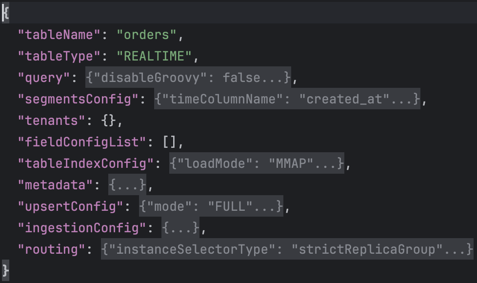
The configuration of tbe table is more involved than the schema so we’ll go over it one key at a time. We begin by specifying the tableName as “orders”. This matches the name of the schema. We specify tableType as “REALTIME” since the data we’re going to ingest comes from a Kafka topic. The query key specifies properties related to query execution. The segmentsConfig key specifies properties related to segments like the time column to use for creating a segment. The tenants key specifies the tenants for this table. A tenant is a logical namespace which restricts where the cluster processes queries on the table. The tableIndexConfig defines the indexing related information for the table. The metadata key specifies the metadata for this table. The upsertCconfig key specifies configuration for upserting into the table. The ingestionConfig key defines where we’d be ingesting data from and what field-level transformations we’d like to apply. The routing key defines properties that determine how the broker selects the servers to route.
The part of the configuration we’ll specifically look at is the ingestionConfig and upsertConfig. First, ingestionConfig.
In the ingestionConfig we specify the the Kafka topics to read from. In the snippet above, we’ve specified the “orders” topic. We also specify field-level transformations in transformConfigs. Here we extract the id, source, and created_at fields from the JSON payload generated by Debezium.
With the schema and table defined, we’ll POST them to the appropriate endpoints using curl. The following two commands create the schema followed by the table.
Once the table is created, it will begin ingesting data from the “orders” Kafka topic. We can view this data by opening the Pinot query console. Notice how the source column contains the entire “after” payload generated by Debezium.
That’s it. That’s how to stream data using Debezium into Pinot.