In the previous post we looked at nullability and how Pinot requires that a default value be specified in place of an actual null. In this post we’ll begin looking at how to query data stored in Pinot. We’ll begin by querying Pinot using its API and query console. Then, we’ll query Pinot using Trino. We’ll use Trino’s query federation capability to create views and tables on top of the data that’s stored in Pinot.
Getting started
Pinot provides an SQL interface for writing queries that’s built on top of the Apache Calcite query parser. It ships with two query engines - the single-stage engine called v1 and the multi-stage engine called v2. The single-stage engine allows writing simpler SQL queries that do not involve joins or window functions. The multi-stage query engine allows more complex queries involving joins on distributed tables, window functions, common table expressions, and much more. It’s optimized for in-memory processing latency. Queries can be submitted to Pinot using the query console, REST API, or Trino. When querying Pinot using either the API or query console, we need to explicitly enable the multi-stage engine.
We’ll begin by writing SQL queries and submitting them first using the API and then using the query console. For queries that require a lot of data shuffling or data that spills to disk, it is recommended to use Presto or Trino. Let’s start by writing a simple SQL query that retrieves the user agent from the orders table. The SQL query to do this is given below.
1 | SELECT user_agent FROM orders LIMIT 1; |
We’ll create a file called query.json which contains the payload that we’ll POST to Pinot. It contains the SQL query and options to indicate to Pinot that we’d like to use the multi-stage engine to execute the query. The content of the file is given below.
1 | { |
We can now POST this payload to the appropriate endpoint using curl.
1 | curl -s -d @query.json localhost:9000/sql | jq ".resultTable" |
The response is returned as a large JSON object but the part we’re interested in is stored in the key called resultTable. It contains the names of the columns returned, the values of the columns, and their datatypes. The following shows the result returned for the query that we’ve submitted above.
1 | { |
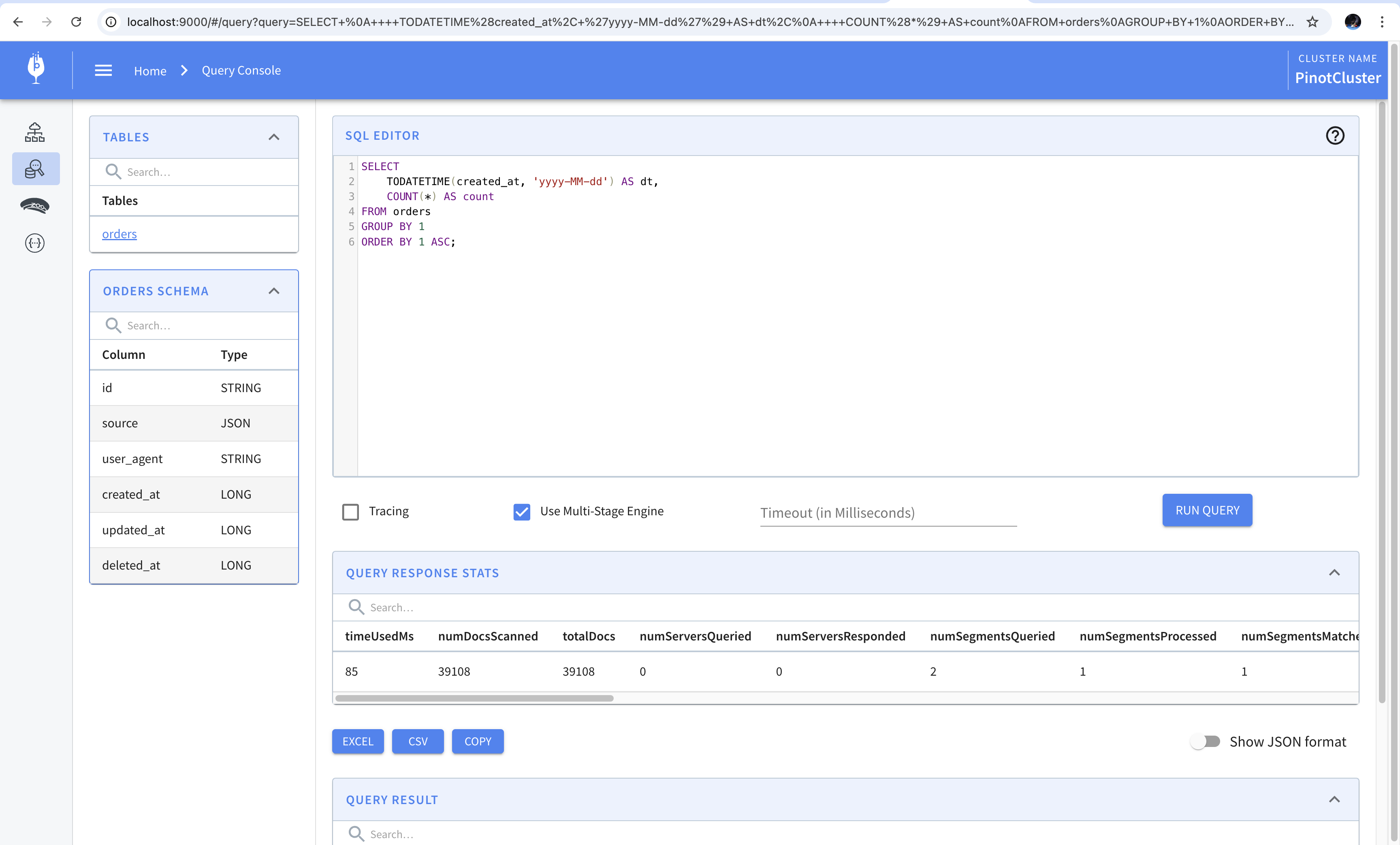
We’ll now look at writing SQL queries using the query console. Let’s write a SQL query which counts the number of orders placed each day. To do this, we’d have to convert the created_at column from milliseconds to date and then run a group by to find the count of the orders that have been placed. The following query gives us the desired result.
1 | SELECT |
We can run this in the console using the single-stage engine since it is one of the simpler queries. To do this, we’ll paste the query in the query console and leave the “Use Multi-Stage Engine” checkbox unchecked. The result of running the query is shown in the screenshot below.

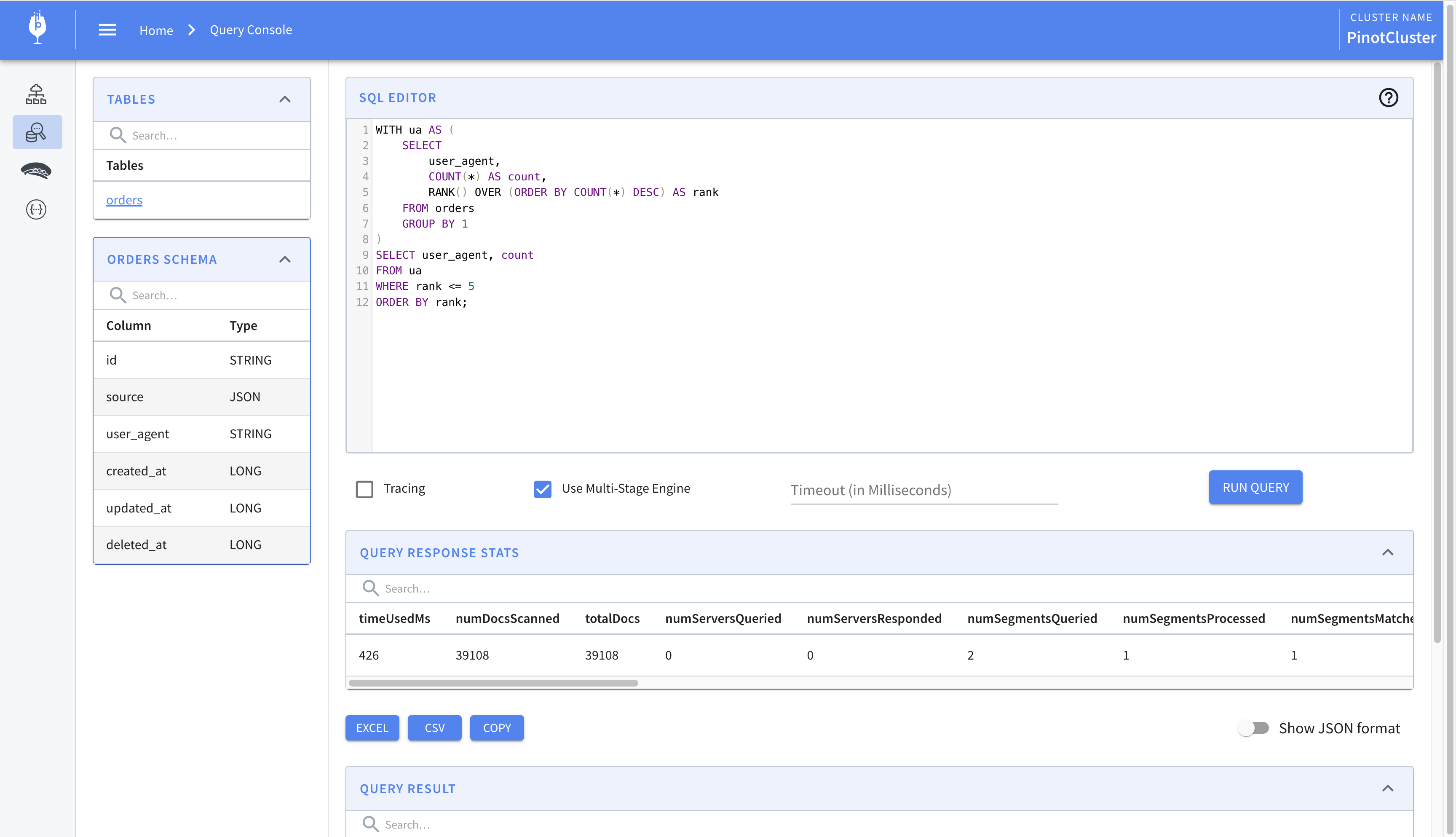
We’ll now modify the query so that it requires the multi-stage engine. Using features of SQL language like window functions, common table expressions, joins, etc. requires executing the query using the multi-stage engine. We’ll write a query which finds the top five user agents and ranks them. This requires using common table expressions, and window functions and is the perfect candidate for using the multi-stage engine. The query is shown below.
1 | WITH ua AS ( |
The result of running this query is shown below. Notice how the checkbox to use the multi-stage engine is checked.

Having seen how to query Pinot using the API, and the query console with either single-stage or multi-stage engine, we’ll move on to querying Pinot using Trino. We’ll begin by connecting to Trino using its CLI utility and create a catalog which connects to our Pinot instance. Then, we’ll run queries using Trino. We’ll also see how we can leverage query federation provided by Trino to connect to AWS Glue and create views and tables on top of the data stored in Pinot.
Let’s start by connecting to Trino. The following command shows how to connect to the Trino instance running as a Docker container using its command-line utility. You can follow the instructions mentioned in the official documentation to setup the CLI.
1 | ./trino http://localhost:9080 |
Every database in Trino that we’d like to connect to is configured using a catalog. A catalog is a collection of properties that specify how to connect to the database. We’ll begin by creating a catalog which allows us to query Pinot.
1 | CREATE CATALOG pinot USING pinot |
The CREATE CATALOG command creates a catalog. It takes the name of the catalog, which we’ve specified as pinot, and the name of the connector which connects to the database, which we’ve also specified as pinot. The WITH section specifies properties that are required to connect to the database. We’ve specified the URL of the controller. Once the catalog is created, we can begin querying the tables in the database. The tables in Pinot are stored in the default schema of the pinot connector. To be able to query these, we’ll have to USE the catalog and schema. The following command sets the schema for the current session.
1 | USE pinot.default; |
To view the tables in the current schema, we’ll execute the SHOW TABLES command.
1 | trino:default> SHOW TABLES; |
Let’s build upon the query that we wrote previously which calculates the count of the orders placed on a given day. Let’s say we’d like to find the percentage change between the number of orders placed on a given day and the day prior. We can do this using the LAG window function which will allow us to access the value of the prior row. The following query shows how to calculates this.
1 | WITH FUNCTION div(x DOUBLE, y DOUBLE) |
There’s a lot going on in the query above so let’s break it down. We begin by defining an inline function called DIV which performs division on two numbers. The reason for writing this function is that the division operator in Pinot returns the integer part of the quotient. To get the quotient as a decimal, we’d have to cast the values to DOUBLE. The function does just that. In the common table expression, we calculate the number of orders placed each day. Finally, in the SELECT statement, we find the number of orders placed on the day prior using the LAG window function.
Running the query gives us the following result.
1 | dt | count | prev_count | pct |
Let’s now say that we’d like to run the query frequently. Perhaps we’d like to display the table in a visualization tool. One way to do this would be to store the query as a view. However, Pinot does not support views. We’d have to work around this by relying on Trino’s query federation to write the result to another data store which supports creating views. For the sake of this post, we’ll use AWS Glue as a replacement for HDFS.
Let’s start with creating a Hive catalog in which we use S3 as the backing store.
1 | CREATE CATALOG hive USING hive |
In the query above, we’re creating the Hive catalog which we’ll use to create and store datasets. Since we’re storing files in S3, we need to specify the region and its S3 endpoint. You’d have to replace the keys with those of your own if you’re running the example locally.
Once we create the catalog, we’ll have to create the schema where datasets will be stored. Schemas are created with CREATE SCHEMA command and require that we provide a path in an S3 bucket where the files will be stored. The query below shows how to create a schema named views.
1 | CREATE SCHEMA hive.views |
Once the schema is created, we can persist the query or its results for quicker access. In the query that follows, we create a view on top of Pinot.
1 | CREATE VIEW hive.views.daily_orders AS |
We can query the view once it is created. This allows us to save the queries so that they can be referenced in data visualization tools. In the view above, we’ll get the realtime difference between orders placed since Pinot will be queried every time we select from the view. A small caveat to note is that views cannot store inline functions so we had to cast one of the operands in the division operation to double manually.
To see this in action, we’ll run the data generation script one more time and then query the view. We can see that the counts for orders placed today, yesterday, and day before yesterday increase after the script runs.
1 | trino> SELECT * FROM hive.views.daily_orders; |
Creating views like this provides us with a way to save queries that we’d like to run frequently. As we’ll see in later posts, these can also be referenced in data visualization tools to provide realtime analytics.
That’s it on how to run SQL on Pinot.