In the previous post we looked at computing the Fibonacci series both with and without dynamic programming. In this post we’ll look at another example where dynamic programming is applicable. The example is borrowed from ‘Introduction to Algorithms’ by CLRS and implemented in Python. By the end of this post we’ll try to develop an intuition for when dynamic programming applies.
Rod Cutting
The problem we are presented with is the following: given a steel rod, we’d like to find the optimal way to cut it into smaller rods. More formally, we’re presented with a rod of size n inches and a table of prices pi. We’d like to determine the maximum revenue rn that we can obtain by cutting the rod and selling it. If the price pn of the rod of length n is large enough, we may sell the rod without making any cuts.
The table of prices that we’ll work with is given below.
| length i | 1 | 2 | 3 | 4 | 5 | 6 | 7 | 8 | 9 | 10 |
|---|---|---|---|---|---|---|---|---|---|---|
| price pi | 1 | 5 | 8 | 9 | 10 | 17 | 17 | 20 | 24 | 30 |
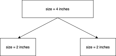
Consider a rod of length 4 inches. The maxium revenue we can obtain is 10 by cutting the rod into two parts of length 2 inches each.

Given a rod of n inches, we may sell it uncut or we may sell it by cutting it into smaller pieces. Since we do not know the size of the cuts to make, we will have to consider all possible sizes. Once we make a cut of size
It states that the revenue rn is the maximum revenue obtained by considering all cuts of size
1 | def rod_cut(p: list[int], n: int) -> int: |
We can verify the results by calling the function for a rod of size 4 and passing the table of prices.
1 | p = [0, 1, 5, 8, 9, 10, 17, 17, 20, 24, 30] |
The recursive version, however, does redundant work. Consider the rod of size n = 4. We will have to consider cuts of size
We can use dynamic programming to solve this problem by modifying the rod_cut function as follows.
1 | def rod_cut(p: list[int], t: list[int | None], n: int) -> int: |
Notice how we’ve introduced a table t which stores the maximum revenue obtained by cutting a rod of size n. This allows us to reuse previous computations. We can run this function and verify the result.
1 | t = [None] * 11 |
The question that we’re left with is the following: how did we decide that the problem could be solved with dynamic programming? There are two key factors that help us in deciding if dynamic programming can be used. The first is overlapping subproblems and the second is optimal substructure.
For a dynamic programming algorithm to work, the number of subproblems must be small. This means that the recursive algorithm which solves the problem encounters the same subproblems over and over again. When this happens, we say that the problem we’re trying to solve has overlapping subproblems. In the rod cutting problem, when we try to cut a rod of size 4, we consider cuts of size
The second factor is optimal substructure. When a problem exhibits optimal substructure, it means that the solution to the problem contains within it the optimal solutions to the subproblems; we build an optimal solution to the problem from optimal solutions to the subproblems. The rod-cutting problem exhibits optimal substructure because the optimal solution to cutting a rod of length
Moving on. So far our algorithm has returned the optimal value of the solution. In other words, it returned the maximum revenue that can be obtained by optimaly cutting the rod. We often need to store the choice that led to the optimal solution. In the context of the rod cutting problem, this would be the lengths of the cuts made. We can do this by keeping additional information in a separate table. The following code listing is a modification of the above function with an additional table s to store the value of the optimal cut.
1 | def rod_cut(p: list[int], s: list[int | None], t: list[int | None], n: int) -> int: |
In this version of the code, we store the size of the cut being made for a rod of length n in the table s. Once we have this information, we can reconstruct the optimal solution. The function that follows shows how to do that.
1 | def optimal_cuts(s: list[int | None], n: int) -> list[int]: |
Finally, we call the function to see the optimal solution. Since we know that the optimal solution for a rod of size 4 is to cut it into two equal halves, we’ll use
1 | n = 4 |
That’s it. That’s how we can use dynamic programming to optimally cut a rod of size