In one of the previous posts we looked at the assumptions underlying the classic linear regression model. In this post we’ll take a look at the Gauss-Markov theorem which uses these assumptions to state that the OLS estimators are the best linear unbiased estimators, in the class of linear unbiased estimators.
Gauss-Markov Theorem
To recap briefly, some of the assumptions we made were that:
- On average, the stochastic error term is zero i.e.
. - The data is homoscedastic i.e. the variance / standard deviation of the stochastic error term is a finite value regardless of
. - The model is linear in parameters i.e.
and have power 1. - There is no autocorrelation between the disturbance terms.
The Gauss-Markov theorem states the following:
Given the assumptions underlying the CLRM, the OLS estimators, in the class of linear unbiased estimators, have minimum variance. That is, they are BLUE (Best Linear Unbiased Estimators).
We’ll go over what it means for an estimator to be best, linear, and unbiased.
Linear
The dependent variable
Unbiased
This means that on average, the value of the estimator is the same as the parameter it is estimating i.e.
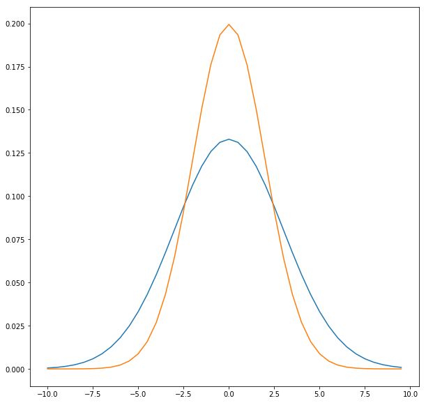
Best
This means that among the class of linear estimators, the OLS estimators will have the least variance. Consider the two normal distributions shown in the graph above for two linear, unbiased estimators
Finito.